Dont’t decay the learning rate, increase the batch size

Original paper: https://arxiv.org/abs/1711.00489

Authors: Samuel L. Smith, Pieter-Jan Kindermans, Chris Ying, Quoc V. Le (Google Brain)

Practical view of Generalization

• 기존 연구들은 어떻게 해야 generalization이 되는지를 많이 제안했었음.
  • Imagenet challenge에서 제안된 여러 구조들이 generalization이 잘 되는 구조와 hyper parameter setting들을 전부 다 포함
  • Generalization 성능이 좋은 구조와 hyper parameter들을 유지하면서 응용하려면?
• 본 논문에서는 generalization에 크게 영향을 끼치는 learning rate, batch size에 대해 다룸

Batch size in the Deep learning

• Batch size가 크면 연산이 효율적(빠른 학습 가능)
• Batch size가 작으면 generalization이 잘 됨
• 연산 효율을 좋게 하면서 generalization을 잘 시키는 방법에 대해 본 논문에서는 연구

Batch size and Generalization

• Imagenet을 1시간 안에 학습 시키는 논문
  • P.Goyal et al. (2017), “Accurate, Large Minibatch SGD: Training ImageNet in 1 Hour”
• 위 논문에서 주요하게 사용한게 Linear scaling rule
  • Batch size 크기에 비례해서 learning rate를 조절해야한다는 rule
  • Batch size가 2배가 되면, learning rate도 2배가 되어야 함

Contribution

• Learning rate decaying 하는게 simulated onnealing하는것과 비슷함.
  • Simulated annealning 이론을 기반으로 learning rate decaying에 대해 설명.
• Linear scaling rule / learning rate를 decaying 하지말고, batch size를 늘리자
• SGD momentum coefficient 또한 batch size 조정하는 rule에 포함 시킬 수 있음

위의 방법들을 사용하여 2500번의 parameter update로 ImageNet dataset을 traning했음(Inception-Resnet-V2)

Noted items

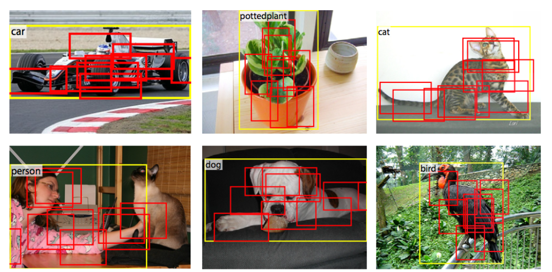
• Batch size와 generalization의 관계
  • Sharp한 minimum이 generalization에 나쁘다고 표현됨
  • 그렇지 않은(broad) minimum은 generalization이 잘 된다고 봄
  • SGD가 batch size가 작으면 SGD가 갖는 noise 성분이 커지게 됨
  • 따라서 자연스럽게 broad한 minimum을 갖게 됨
  • 즉, Sharp minimum -> bad to generalization / Broad minimum -> good to generalization
• SGD와 batch size의 관계에서 보는 generalization의 영향
  • SGD W/O noise: $\Theta_{t+1} \leftarrow \Theta_{t} + \alpha_{t}\nabla\Theta$
  • SGD W/ noise: $\Theta_{t+1} \leftarrow \Theta_{t} + \alpha_{t}(\nabla\Theta + N(0, \sigma^2_t))$
  • Noise term: $N(0, \sigma^2_t)$ -> Noise가 minima를 general하게 만들어줌
• 작은 batch 사이즈
  • Weight parameter 업데이트 횟수가 많음
  • SGD가 많은 noise component를 가짐
  • 더 broad한 minima를 가짐

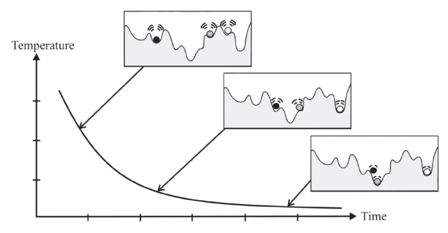
• Simulated annealing
  • Optimum을 찾는데 gradient를 이용해서 하는것이 아니고, Random하게 움직여서 값이 좋아지면 그 방향으로 가는 optimization
  • Gradient descent와 같이 local minima에 빠지는 문제를 해결하기 위해 temperature라는 option를 이용하여 조금 움직여서 결과가 좋아지지 않더라도 temperature option에 의해 그 결과를 accept함.
  • 사진에서, 움직였는데 공이 조금 더 위로 올라가도 그냥 올라가는것을 의미
  • SGD에서 noise가 하는 역활과 같이 temperature가 local minima를 빠져나가게 함
  • 시간 갈수록 SGD에서 learning rate를 decaying하듯이 temperature를 조절하여 global minima에 도달할 수 있도록 함
• Momentum
  • Gradient descent 최적화 알고리즘의 한 종류
  • 종류로는 momentum, Nestrov momentum이 많이 쓰임
  • 모멘텀 알고리즘은 누적된 과거 gradient가 지향하고 있는 어떤 방향을 현재의 gradient에 보정하려는 방식
  • 일종의 관성가속도 정도로 이해하면 쉬움

Stochastic gradient descent and Convex optimization

• Convergence conditions of SGD
  • Convex surface(Convex loss function)에서 수렴하는 조건(SGD가 수렴하기 위한 조건)
  • For fixed batch size

1. $$\sum^\infty_{i=1}\epsilon_i = \infty$$
2. $$\sum^\infty_{i=1}\epsilon^2_i < \infty$$

• 1에서, 수렴하기 위해서는 lr의 sum이 무한대
• 2에서, lr의 제곱의 모든 sum이 유한해야 함
• 직관적으로
  • 1에서, 시작 point와 global optimum이 얼마나 멀든지 간에 다가갈 수 있어야 함
  • 2에서, SGD가 noise가 있으니 그 noise에 의해 optimum 근처에서 진동 할 때, noise가 있음에도 수렴해야 할 조건
• Interpretation of SGD for various batch size
  • 위의 논의를 다양한 batch size에 대해서도 확장

• $\frac{dC}{dw}$은 Cost function의 gradient, $\eta(t)$은 gradient를 의미

• 위 식에서 $\eta(t)$(SGD를 쓰기때문에 발생하는 noise)의 variance가 $<\eta(t)\eta(t')>=gF(w)\delta(t-t')$ 가 된다고 분석(mean = 0)

• Noise scale $g$
  • $$g=\epsilon(\frac{N}{B}-1)$$
  • $\epsilon$은 learning rate, $N$은 전체 traning data size, $B$는 batch size를 의미
  • $g$를 수학적(stochastic differential equation)으로 풀어서 왼쪽의 관계가 나옴(과정은 다른논문)
  • 결론적으로, SGD를 사용함으로써 생기는 variance가 위의 식에 비례
  • 위의 식이 linear scaling rule을 의미
  • 보통 $N»B$이므로, -1항은 무시 가능하여 아래의 식으로 근사화가 가능
  • $$g\approx\epsilon\frac{N}{B}\longrightarrow g\propto\frac{\epsilon}{B}$$
  • Batch size를 조절하면 똑같이 lr($\epsilon$)을 비례해서 키워줘야 하고, SGD로부터 발생한 noise(random fluctuation)가 동일(일정)하게 유지 될 수 있다(linear scaling rule)
  • 이로부터 generalization이 유지가 된다고 생각 할 수 있음
• Random fluctuation이 generalization에 가장 영향을 크게 미침(일정하게 유지되어야 함)
• 실험적인 결과도 Random fluctuation이 일정하게 유지 될 때 가장 좋았음
  • $g$의 식에서 -1을 무시하기 위해서는 batch size가 너무 많이 커지면 안됨
  • $B\approx\frac{N}{10}$정도까지는 가능하지만, 더 커지면 -1항을 무시 할 수 없게 됨

Simulated annealing and the generalization gap

• Simulated annealing
  • learning rate를 decaying하는 dynamics가 simulated annealing과 동일
  • Lr을 decaying하는것과 같이 simulated annealing도 random flucuation을 줄임
  • Simulated annealing이라는 개념을 가져와서 lr의 decaying을 정당화 시킴(lr decaying 하는것이 generalization에 좋다)
  • Simulkated annealing이 random flucuation을 줄이듯, lr decaying하는것이 좋음
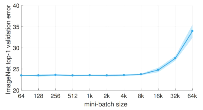
• Generalization gap -> batch size가 작으면 generalization이 잘 된다
  • Large batch size보다 test 결과가 더 좋다
  • SGD에 들어가는 noise가 sharp minima를 벗어나 generalization에 좋은 broad minima를 찾는데 도움이 됨
  • Simulated annealing이 annealing을 천천히 하는것이 sharp minima에 converge하고, 급격히 하는게 broad minima를 찾는데 효과적
  • 보통 lr 조절 시 exponential 하게 하지 않고, 유명한 논문들에서 30, 60, 90 epoch 등에서 1/10 수준으로 확 decaying하는것이 simulated annealing에서 정당화 시키는 내용
  • Simulated annealing에서도 확확 annealing 하는게 더 broad한 minima를 찾는데 도움이 됨

The effective learning rate and the accumulation variable

• Noise scale of random fluctuation in the SGD with momentum dynamics
  • $$g=\frac{\epsilon}{1-m}(\frac{N}{B}-1)\approx\frac{\epsilon N}{B(1-m)}$$
  • 즉, momentum ($m$: momentum coefficient)함수 쓸 때 $g$는 위의 관계를 가짐
  • 하지만, 실제로는 결과가 좋지 않게 나옴
• Problem analysis
  • $$\Delta A=-(1-m)A+\frac{d\hat{C}}{dw}$$
  • $$\Delta w=A\epsilon$$
  • 이유: momentum이 처음에 0으로 초기화
  • 즉, 0에 초반에 biased 되어 있게 되므로 weight update가 원래 계산보다 더 적게 수행됨
  • $g=\approx\frac{\epsilon N}{B(1-m)}$이므로, $g$를 유지하면서 batch size($B$)를 키우려면 momentum ($m$)을 키워야 함
  • Momentum을 높이면 weight update가 초반에 잘 되지 않는 문제 발생
  • 그 해결책으로 Training epoch를 더 해야함

Experiment 환경

• Cifar-10 dataset
  • 50,000 images for training
  • $B_{max}=5120$ (by $N\gg B$, $1/10$ rule)
  • 학습 시 batch size를 증가시키며 진행하다 $B_{max}$ 되면 lr을 decaying
• ImageNet dataset
  • 1.28 million images
  • $B_{max}=65536$
• Ghost batch normalization 사용
  • Batch normalization 또한 batch size가 바뀜에 따라 noise의 양이 변하게 됨 (parameter update 횟수 변경에 의한 batch size 증가 시 전체 noise 감소)
  • 따라서, 전체가 아닌 Sampled data에 대해서만 Statistics(variance, mean)을 계산하여 batch normalization을 수행

Simulated annealing in Wide ResNet

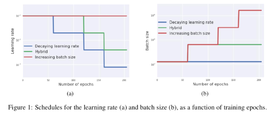
• Three scheduling strategies (Cifar-10 datset)
  • Lr decay factor: 5, 3가지 Scheduling rule 사용
  • 파란 선: 일반적인 방법
  • 초록 선: 초반에는 Batch size 증가, 그다음엔 lr decaying
  • 빨간 선: lr을 유지하면서 batch size를 5배씩 증가

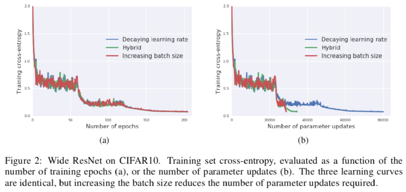
• Training loss curve
  • Loss curve가 동일하다는것을 보여주려 함
  • (a): Loss curves are identical
  • (b): Increasing batch size strategy significantly reduces the number of parameter updates
  • Batch size가 커지는 경우 parameter update 수는 줄어들어 더 빠른 학습이 가능
  • Batch size를 조절하는 것이 random fluctuation에 끼치는 영향이 같으므로 generalization이 똑같이 잘 된다(Traning)

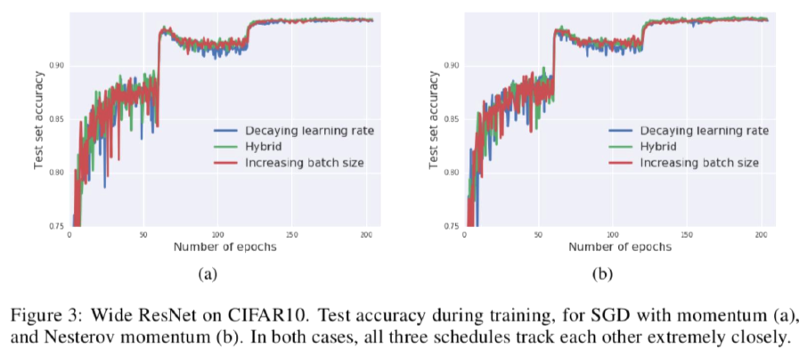
• Test loss curves A(Test set에 대한 accuracy)
  • (a): SGD with momentum, (b): SGD with Nestrov momentum
  • 다른 momentum을 사용하더라도 결과는 거의 동일한것을 알 수 있음

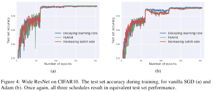
• Test loss curves B
  • (a): Vanilla SGD, (b): Adam
• 결국 논문에서 제안하는 방법과 기존 방법의 차이에 대한 성능 변화가 적음

Increasing the effective learning rate

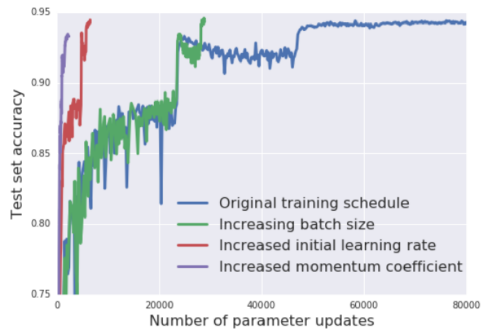
• Momentum coefficient를 변화시킨 실험 결과
  • Default settings: initial LR 0.1, decay factor 5, momentum 0.9, batch size 128
  • “Increasing batch size”: increasing batch size by a factor 5
  • “Increased initial learning rate”: initial LR 0.5, initial batch size 640, increasing batch size
  • “Increased momentum coefficient”: initial LR 0.5, momentum 0.98, initial batch size 3200
  • The final result of “Increased momentum coefficient” is 93.3%, lower than original 94.3%
  • 결과적으로 increased momentum coefficient는 결과가 좋지 않음(1%정도 하락)
  • 논문에선 보라색 그래프(제일 좌측)가 아직 수렴하지 않았으므로 더 학습 할 경우 정확도가 개선 될 것이라 판단하나 실험적으로 내용을 넣진 않음…

Training ImageNet in 2500 parameter updates

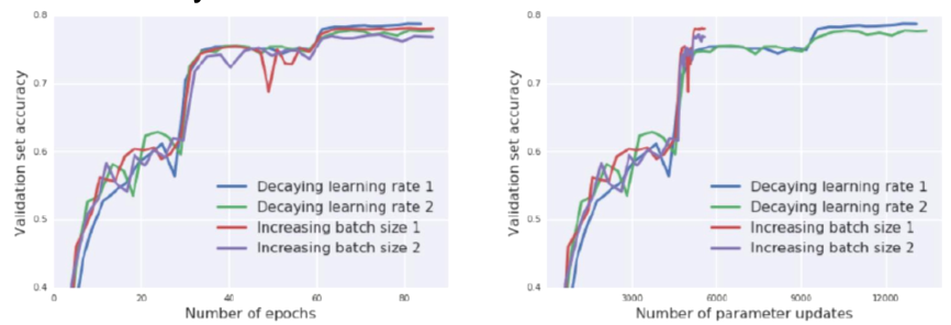
• Control batch size only (ImageNet dataset)
  • 실험 1, 2는 두 실험 간의 variance를 보이기 위하여 두 번을 수행
  • Trained Inception-ResNet-V2
  • Ghost batch size 32, initial LR 3.0, momentum 0.9, initial batch size 8192
  • Increase batch size only for first decay step
  • The result are slightly drops, form 78.7% and 77.8% to 78.1% and 76.8%, the difference is similar to the variance
  • Reduced parameter updates from 14,000 to below 6,000
  • 결과가 조금 안좋아짐. 논문에선 원래 실험 자체 variance가 있으니 그 variance 안에 들어가므로 상관이 없다고 주장…
  • 하지만 실제로는 1%정도의 정확도 하락을 보임

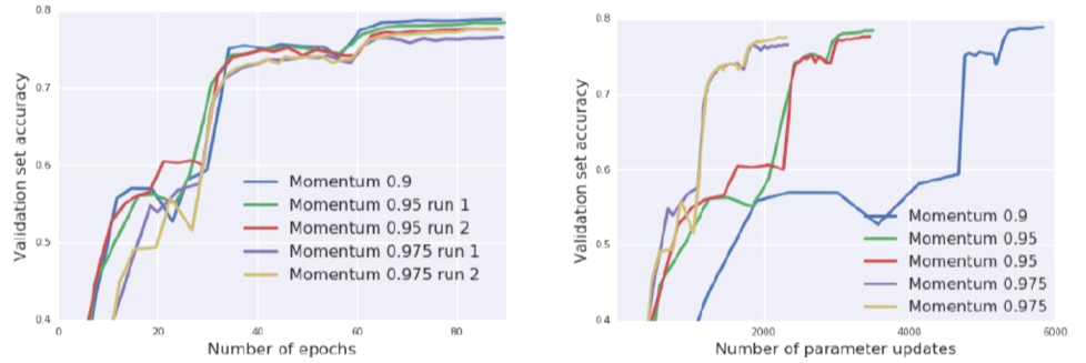
• Control batch size and momentum coefficient
  • Initial LR 3.0 and Ghost batch size 64
  • “Momentum 0.9”: initial batch size 8192
  • “Momentum 0.95”: initial batch size 16384
  • “Momentum 0.975”: initial batch size 32768
  • Momentum coefficient 조절 시 실험 결과가 조금씩 나빠짐
  • Batch size는 늘리고, 거기에 momentum까지 조절

Conlusion

• Scaling rule

• 더 빠른 학습을 수행
  • Large batch size와 momentum을 증가시킴
  • 더 낮은 accuracy loss
• Inception-ResNet-V2를 사용해 ImageNet datset에 대해 2500번의 weight parameter update만을 가지고 77%의 정확도를 달성

• [참고 글]

https://www.youtube.com/watch?v=jFpO-E4RPhQ

Baekjoon 알고리즘 문제풀기

[2739] 구구단

문제

• 입력받은 수의 구구단을 출력

정답

a = int(input())

for j in range(1,10):
    print('%d * %d = %d'%(a, j, a*j))

[2438] 별 찍기 - 1

문제

• 입력 된 숫자만큼의 별을 출력한다.

• print('문자', end="")로 개행 없는 출력을 이용한다.

정답

a = int(input())

for j in range(1, a+1):
    for k in range(0, j):
        print('*', end="")
    print('')

[2439] 별 찍기 - 2

문제

• 입력 된 숫자만큼의 별을 우측 정렬하여 출력한다.

• print(string.rjust(length, "char")) 를 이용하여 우정렬 출력을 한다.

정답

a = int(input())
star = str('')
for j in range(1, a+1):
    star = str('')
    for k in range(0, j):
        #print('*', end="")
        star = str(star) + str('*')
        #print(star)
    print(star.rjust(a," "))

[2440] 별 찍기 - 3 / [2441] 별 찍기 - 4

문제

• 입력 된 숫자만큼의 별을 감소시키며 출력한다

• for(num1, num2, num3): 을 이용하여, num1의 숫자에서 num2의 숫자로 num3만큼씩 증/감 가능한 것을 이용한다.

정답

a = int(input())

for j in range(a, 0, -1):
    for k in range(0, j):
        print('*', end="")
    print('')

a = int(input())
star = str('')
for j in range(a, 0, -1):
    star = str('')
    for k in range(0, j):
        star = str(star) + str('*')
    print(star.rjust(a," "))

[1924] 2007년

문제

• 2007년 x월 y일에 대한 요일을 맞추는 문제

정답

m, d = map(int, input().split())
weeks = ['SUN', 'MON', 'TUE', 'WED', 'THU', 'FRI', 'SAT']
days = [0, 31, 28, 31, 30, 31, 30, 31, 31, 30, 31, 30, 31]

cnt_d = 0

for cnt_m in range(0, m):
    cnt_d += days[cnt_m]

cnt_d += d

remain_w = cnt_d%7
print(weeks[remain_w])

[11721] 열 개씩 끊어 출력하기

문제

• 알파벳을 10개씩 끊어서 출력한다.

정답

a = str(input())
cnt = 0
for j in range(0, len(a)):
    print(a[j], end="")
    cnt+=1
    if(cnt%10==0):
        print('')
print('')

[15552] 빠른 A+B

문제

• 제한 시간(1초) 이내에 빠른 덧셈 연산을 수행한다.
• 첫 줄에 덧셈 연산을 할 횟수가 주어지고, 이어서 연산을 할 두 수가 주어진다.

• 출력은 한번에 하거나 입력을 받은 후 즉시 출력되도 상관 없다.

• 느린 파이썬 input()을 사용하는 대신, sys 라이브러리의 sys.stdin.readline().rstrip()을 이용한다.
• .rstrip()의 경우엔 마지막 개행까지 입력되는 것을 막아준다.

정답

import sys

a = sys.stdin.readline().rstrip()

for j in range(0, int(a)):

    b, c = map(int, sys.stdin.readline().rstrip().split())
    print(b+c)

Jekyll 테마 Github blog에 MathJax를 이용한 수식 입력 가능하게 하기

Gihub를 이용한 blog는 기본적으로 수식 입력이 불가능하다. (오직 이미지 형태로만 업로드 가능 ㅠㅠ) 그래서 손쉽게 Github상에서 Inline, outline 수식 입력이 가능하도록 해주는 MathJax를 설치했다.

설치방법

Jekyll 테마가 적용된 Github blog에서 /_layouts/post.html에 <article> 바로 위에 아래의 줄을 붙여넣기한다.

    <script type="text/x-mathjax-config">
    MathJax.Hub.Config({tex2jax: {inlineMath: [['$','$'], ['\\(','\\)']]}});
    </script>
    <script type="text/javascript" src="http://cdn.mathjax.org/math...">
    </script>

위 스크립트가 적용된 예시는 아래와 같다.

테스트를 위해 아래와 같은 수식을 적어서 포스팅해보자.

$\sum_{i=0}^n i^2 = \frac{(n^2+n)(2n+1)}{6}$ (Inline 수식용)

$$\sum_{i=0}^n i^2 = \frac{(n^2+n)(2n+1)}{6}$$ (Outline 수식용)

스크립트가 제대로 설치되었다면 블로그에선 아래의 사진과 같이 수식이 보인다.

사용방법

수식 적용방법은 inline의 경우 $[수식]$, outline의 경우 $$[수식]$$을 이용한다. 문법의 내용은 다음의 사이트들을 참고한다.

• https://en.wikibooks.org/wiki/LaTeX/Mathematics (LaTex docs)
• https://johngrib.github.io/wiki/mathjax-latex/ (간단한 사용예시)
• http://detexify.kirelabs.org/classify.html (모르는 기호를 LaTex 문법으로 맞춰 제안)
• https://latexbase.com/ (온라인 LaTeX 수식 확인 가능 사이트 -상당히 유용!)

• [참고 글]

https://helloworldpark.github.io/jekyll/update/2016/12/18/Github-and-Latex.html

Baekjoon 알고리즘 문제풀기

[1000] A+B / [1001] A-B / [10998] AxB / [1008] A/B / [10869] 사칙연산

문제

• 두 정수 A와 B를 받고, 연산하여 출력하는 프로그램

• 다중 입력을 원할경우 map(형식, input().split())을 활용한다.

정답

a, b = map(int, input().split())
print(a+b)
print(a-b)
print(a*b)
print('%0.9'%(a/b))
print(int(a/b))
print(a%b)

[10172] 개

문제

• 아래 주어진 개를 출력하는 프로그램

• 파이썬에서 ‘\‘를 출력하고자 할때는 ‘\\‘로 입력해야 한다.
• 줄 개행이 포함된 출력을 원할경우 print('''내용''')을 이용한다.

|\_/|
|q p|   /}
( 0 )"""\
|"^"`    |
||_/=\\__|

정답

print('''|\\_/|
|q p|   /}
( 0 )"""\\
|"^"`    |
||_/=\\\\__|''')

[11718] / [11719] 그대로 출력하기

문제

• 주어진 입력 그대로 출력한다.
• 최대 100줄, 한 문장은 100자를 넘지 않는다.

정답

cnt = 1
while True:
    print(input())
    cnt += 1
    if (cnt == 100):
        break

• 하지만 계속 런타임 에러가 나서 아래의 코드로 제출했다…

  while True:
    try:
        print(input())
    except EOFError:
        break
  

[10430] 나머지

문제

• (A+B)%C는 (A%C + B%C)%C 와 같을까?
• (A×B)%C는 (A%C × B%C)%C 와 같을까?

정답

A, B, C = map(int, input().split())
print((A+B)%C)
print((A%C + B%C)%C)
print((A*B)%C)
print((A%C*B%C)%C)

[2839] 설탕배달

문제

• 주어진 설탕 무게를 3, 5 kg 봉지에 나눠 담어야 한다.
• 단, 갯수는 최대한 적게 되도록 한다.(18kg일 경우 3kg 6개가 아닌 5kg 3개, 3kg 1개로 총 4개)

• 단, 정확하게 N개의 봉지로 나눌 수 없는경우엔 -1을 출력한다.

• 처음에 문제를 잘못 이해해서 애를 많이 먹었다.
• 최대한 큰 봉지(5kg)에 담고, 남은 설탕이 3kg봉지에 딱 맞아떨어지지 않게되면 5kg 봉지를 하나씩 깐다.
• 만약 5kg봉지를 다 깟는데도 3kg으로 나눠떨어지지 않는 경우에는 3kg 봉지로 정확히 담을 수 없는 상황이므로 -1을 출력한다.

정답

a = int(input())

f = a//5
fr = a%5
while True:
    t = fr//3
    tr = fr%3
    
    if (tr!=0):
        f -= 1
        fr += 5
    else:
        result = f + int(t)
        break
    if (f<0):
        result = -1
        break

print(result)

Dilated Convolution과 Deformable Convolution

Object detection에 관련된 딥러닝 논문을 읽다 보면 Feature extractor에서 사용되는 다양한 종류의 컨벌루션이 논해진다. 그 중 RFBNet 논문을 읽으며 알게 된 Dilated Convolution과 Deformable Convolution에 대해 간단하게 공부해봤다.

Dilated Convolution

• FCN 개발자들은 dilated convolution 대신 skip layer/upsampling을 사용
  • 기본적인 convolution과 유사
• 아래의 그림에서 빨간 점만을 이용해 convolution을 수행.
  • 이유? 해상도 손실 없이 receptive field 크기 확장 가능

• (a): 1-dilated convolution으로 기존의 일반적인 convolution 연산과 동일
• (b): 2-dilated convolution. 각 빨간점만 convolution 연산에 사용.(나머지는 0으로 채워짐)
  • Receptive field 크기가 7x7 영역으로 커지는 꼴

• (c): 4-dilated convolution. Receptive field 크기가 15x15로 커지는 꼴

• Dilated convolution 사용 시 receptive field가 커지는 효과를 얻을 수 있음.
  • 파라미터 개수(연산량)가 늘어나지 않으며 큰 receptive field를 취할 수 있는 장점이 존재(conv 표현력 대비 연산량 감소)
• ex. 7x7크기의 receptive field에 대해
  • Normal: 49개의 parameters(7*7)
  • Dilated: 9개의 parameters(3*3) -> 나머지는 모두 0으로 채워짐
• Dilated convolution의 이점?
  • Receptive field의 크기가 커짐.
  • Dilation 계수 조정 시 다양한 scale에 대한 대응이 가능 (다양한 scale에서의 정보를 끄집어내려면 넓은 receptive field가 필요하나, dilated conv가 그 문제를 해결)
  • Pooling을 이용한 receptive field의 확장효과를 얻는 CNN보다 양질의 feature map을 얻을 수 있음(표현력이 더 좋음)

• DeepLab 논문의 그림을 참조하여 위쪽이 pooling과 normal convolution을 이용한 결과, 아래가 Dilated convolution을 이용한 결과

Deformalbe Convolution

• 기존의 CNN방식은 기하학적으로 제한적이고 일정한 패턴을 가정한 convolution을 사용하여 복잡한 transformation에서 유연한 대처가 어렵고, 이로 인하여 명확한 한계가 존재
• CNN Layer에서 사용하는 convolution은 receptive field 크기가 항상 같음

• Convolution에서 사용하는 sampling grid에 2D offset을 더한다는 idea에서 출발
• (a)에 offset을 더해(초록 화살표) (b), (c), (d)의 파란 점들처럼 다양한 패턴으로 convolution을 변형시켜 사용 가능=

• Deformable conv에는 일반적인 conv layer말고 다른 conv layer가 존재
• 위의 그림에서 초록 선의 흰색 conv layer가 각 입력의 2D offset을 학습하기 위한 layer
• 여기서 offset은 integer값이 아닌 fractional number이므로 0.5같은 소수 값이 가능
• 실제 계산은 linear interpolation(2D 이므로 bilinear)으로 이루어짐
• Training 과정에서, output feature를 만드는 convolution kernel과 offset을 정하는 convolution kernel을 동시에 학습 할 수 있음
  • 여기서 ‘offset을 정하는 convolution kernel’은 얼마나 어떻게 멀어질지 정하는 convolutiond

• 붉은 점은 deformable convolution filter에서 학습한 offset을 반영한 sampling location
• 초록색은 filter의 output 위치
• 결과적으로, 일정하지 않은 sampling 패턴에 의해 큰 object에 대해서는 receptive field가 더 커진것을 확인 할 수 있음

Deformable ROI Pooling

• ROI Pooling: 크기가 변하는 사각형 입력 region을 고정된 크기의 feature로 변환하는 과정
• Deformable ROI pooling으로 일반적인 ROI Pooling layer와 offset을 학습하기 위한 layer로 구성
• Deformable conv와 다른점은 offset 학습에 convolution이 아니라 fc layer를 사용(이유는 논문에도 안나와있음…)

• Training 과정에서 offset을 결정하는 fc later도 back-propagation을 통해 학습됨(parameter update)

• 입력 ROI(노란색)에 대해 deformable ROI Pooling(붉은색)의 결과.

• ROI에 해당하는 붉은 사각형의 모양이 object의 형대에 따라 다양한 형태로 변형됨

• 지금까지 deep learning 분야의 많은 연구들은 predictor의 weight 값(parameter, w)을 구하는데 초점을 맞춤

• 위 논문들은 어떤 데이터 x를 뽑을 것인가에 대해 초점을 맞춤

• [참고 글]

https://blog.naver.com/PostView.nhn?blogId=laonple&logNo=220991967450&proxyReferer=https%3A%2F%2Fwww.google.com%2F

https://jamiekang.github.io/2017/04/16/deformable-convolutional-networks/