Receptive Field Block Net for Accurate and Fast Object Detection

Original paper: https://eccv2018.org/openaccess/content_ECCV_2018/papers/Songtao_Liu_Receptive_Field_Block_ECCV_2018_paper.pdf

Authors: Songtao Liu, Di Huang, Yunhong Wang (Beihang University)

Implementation code: https://github.com/ruinmessi/RFBNet (Pytorch)

Abstract

• 정확한 object detector들은 ResNet, Inception과 같은 표현력 좋은 CNN backbone 덕분에 성능이 좋지만 연산량이 많기때문에 한계가 명확하다. 반대로 몇몇의 lightweight 모델을 backbone으로 하는 detector들은 real-time으로 구동이 가능하지만 정확도는 낮다는 단점이 존재한다. 본 논문에선 인간의 시각체계를 이용하여 lightweight feature의 표현력을 강화시켜서 정확하고 빠른 object detector를 제안한다. 인간 시각시스템의 Receptive Fields(RFs)의 구조로부터 영감을 받아서, feature의 구별가능성(discriminability)과 robustness을 강화하기 위해 RFs의 size와 편심(eccentricity) 사이의 관계가 고려된 novel한 RF Block (RFB) module을 제안한다. 또한 RFB를 SSD의 앞부분에 추가하여 RFB Net detector를 만들었다. RFB module의 효용성을 확인하기 위해 두 개의 major benchmark를 이용하여 실험을 수행하였으며, 실험 결과 RFB Net이 real-time 연산속도는 유지하면서 very deep detector들의 성능을 뛰어넘는 결과를 확인 할 수 있었다.

1 Intorduction

• In recent years, Region-based Convolutional Neural Networks (R-CNN) [8], along with its representative updated descendants, e.g. Fast R-CNN [7] and Faster R-CNN [26], have persistently promoted the performance of object detection on major challenges and benchmarks, such as Pascal VOC [5], MS COCO [21], and ILSVRC [27]. 이러한 모델들은 2-stage 구조로써 첫 번째에선 detection 문제에 대해 object proposal을 주어진 이미지에서 만들어내며 두번째 phase에선 각 proposal을 CNN based deep feature에 따라 classification한다. It is generally accepted that in these methods, CNN representation plays a crucial role, and the learned feature is expected to deliver a high discriminative power encoding object characteristics and a good robustness especially to moderate positional shifts (usually incurred by inaccurate boxes). 즉, CNN의 표현력이 detector의 성능에 제일 중요하며, CNN이 얼마나 feature를 잘 뽑느냐에 따라 그 성능이 결정되게된다. 이로인해 다양한 연구들이 진행되었다. For instance, [11] and [15] extract features from deeper CNN backbones, like ResNet [11] and Inception [31]; [19] introduces a top-down architecture to construct feature pyramids, integrating low-level and high-level information; and the latest top-performing Mask R-CNN [9] produces an RoIAlign layer to generate more precise regional features. 모든 이러한 방법들은 더 나은 결과를 만들도록 고품질의 feature를 뽑도록 하는 방법이나 고품질의 feature를 뽑기 위해선 많은 연산량이 필요하고 연산비용이 비싸며 이로인해 inference속도가 낮은 deeper neural network를 사용해야한다는 단점이 있다.
• Detection을 고속화하기 위해 위의 single-stage framework가 개발되었으며, 이는 위의 방식들에서 object proposal generation이 제거된 형태다. Yolo[24]나 SSD[22]와 같은 선구자적인 연구들은 real-time으로 연산이 가능하지만 정확도가 떨어지는 경향을 보이며, 심지어 Focal Loss[20]와 같은 SOTA detector에 비해 10~40%의 정확도가 떨어진다. 더 최근의 Deconvolutional SSD (DSSD)[6]과 RetinaNet[20]의 경우 정확도를 상당히 개선시켰으며 2-stage 방식과 견줄정도의 정확도를 보인다. 하지만 이러한 정확도의 개선은 ResNet-101과 같은 매우 깊은 네트워크를 사용하였기때문에 효율에는 한계가 명확하다.

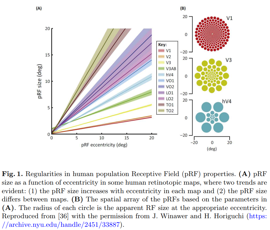
• According to the discussion above, to build a fast yet powerful detector, a reasonable alternative is to enhance feature representation of the lightweight network by bringing in certain hand-crafted mechanisms rather than stubbornly(완고한) deepening the model. 반면에 신경 과학의 여러 연구들에선 인간의 시각 피질에서 population Receptive Field (pRF)의 크기가 그 retinotopic(망막국소) 안의 eccentricity(편심)의 기능이고, 비록 map사이에서 변하더라도 pRF가 각 map에서 eccentricity와 함께 증가하며[36], 이는 그림 1에서 설명되어져있다. 이로인해 중심에 가까운 지역일수록 중요도가 강조되며 조금 이동하더라도 무감각해지게 된다. 이 메카니즘을 이용한 [34, 14, 37]등의 연구가 수행되었고 [1, 38, 19]는 이 pooling scheme을 학습하여 image patch matching에 좋은 성능을 보인다.
• 현재의 딥러닝 모델들은 모통 RFs를 같은 사이즈로 설정하며 동시에 feature map에서 일정한 grid로 샘플링한다. 이는 feature 구별가능성(discriminability)과 더불어 robustness의 손실로 이어진다. Inception[33]은 RFs를 다양한 사이즈로 고려하였고 이 개념을 서로 다른 커널 사이즈를 사용하는 multi-branch CNNs에 적용시켰다. Its variants [32,31,16] achieve competitive results in object detection (in the two-stage framework) and classification tasks. 하지만 Inception에서 사용하는 모든 커널들은 동일한 중심에서 샘플링된다. [3]에서 제안하는 간단한 아이디어는 ASPP라고 하며 이는 multi-scale 정보를 잘 담도록 해준다. It applies several parallel convolutions with different atrous rates on the top feature map to vary the sampling distance from the center, which proves effective in semantic segmentation. 하지만 feature는 같은 커널 사이즈를 사용하는 이전 conv layer에서 온 uniform resolution만을 가지므로 daisy shaped one에 비교하여 결과 feature는 비교적 덜 distinctive(뛰어난, 눈에띄는)한 경향이 있다. Deformable CNN [4] attempts to adaptively adjust the spatial distribution of RFs according to the scale and shape of the object. Deformable CNN이 sampling grid가 flexible하긴 하지만 RFs의 편심(eccentricity)은 고려되지 않았으며 모든 RF의 pixel들이 동등하게 output response에 고려되었고 제일 중요한 정보는 강조되지 않았다는 단점이 존재한다.
  • https://seongkyun.github.io/study/2019/01/02/dilated-deformable-convolution/ 참조

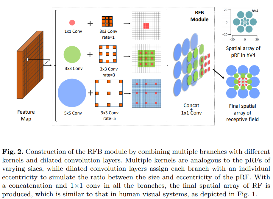
• 인간 시각체계의 RFs 구조에 영감을 받아서 이 논문에서는 새로운 Receptive Field Block(RFB) 모듈을 제안하며, 이는 lightweight CNN에서 학습된 deep feature를 강조하도록 도와주며 이로인해 빠르고 정확한 detection이 가능해진다. 특히 RFB는 해당하는 RFs의 다양한 사이즈에 상응하도록 varying kernels가 적용된 multi-branch pooling을 사용하며 이는 dilated convolution layer에서 편심(eccentricies)을 조절하도록 하는데 적용되었고, 이걸 reshape해서 Figure 2에서처럼 최종 representation을 만들어낸다.
• 본 논문의 main contributions는 다음과 같다.
  1. RFB 모듈을 제안하며, 이는 lightweight CNN network의 deep feature를 강화하도록 하기 위하여 인간 시각 시스템의 RFs의 size와 편심(eccentricity)의 관점에서의 configuration을 시뮬레이션 하기 위함이다.
  2. RFB Net based detector를 제안하고, 이는 SSD의 top convolution layer를 간단히 RFB로 바꾼 형태이며, 이로 인해 연산량을 조절하면서 큰 성능의 향상이 있게 되었다.
  3. RFB Net은 Pascal VOC와 MS COCO dataset에서 SOTA의 결과를 보임과 동시에 real-time 수준으로 동작했으며, RFB의 일반화 성능을 MobileNet[12]에도 적용이 가능했다.

2 Related Work

• Two-stage detector: R-CNN [8] straightforwardly combines the steps of cropping box proposals like Selective Search [35] and classifying them through a CNN model, yielding a significant accuracy gain compared to traditional methods, which opens the deep learning era in object detection. Its descendants (e.g., Fast R-CNN [7], Faster R-CNN [26]) update the two-stage framework and achieve dominant performance. Besides, a number of effective extensions are proposed to further improve the detection accuracy, such as R-FCN [17], FPN [19], Mask R-CNN [9].
• One-stage detector: The most representative one-stage detectors are YOLO [24,25] and SSD [22]. They predict confidences and locations for multiple objects based on the whole feature map. Both the detectors adopt lightweight backbones for acceleration, while their accuracies apparently trail those of top two-stage methods.
• 최근의 DSSD[6]나 RetinaNet[20]과 같은 single-stage detector들은 원래 lightweight backbone를 ResNet-101같이 깊은 구조에 deconvolution[6]이나 Focal Loss[20]과 같은 기술을 적용해서 성능이 two-stage detector만큼 좋아졌다. 하지만 이러한 모델들은 속도가 느리다는 단점이 존재한다.
• Receptive field: 본 논문은 연산량을 너무많이 증가시키지 않으면서 빠른 single-stage detector의 성능을 향상시키기 위한 목적을 가졌다. 따라서 깊은 구조의 backbone을 사용하지 않고 RFB라고 하는 인간 시각시스템의 RFs 메카니즘을 흉내내는 것을 사용하여 lightweight based model의 feature 표현력을 좋게 했다. 사실 몇몇 연구들이 CNN의 RFs에 대해 논했었지만, 대부분의 연구들은 Inception family[33, 32, 31], ASPP[3], Deformable CNN[4] 였다.

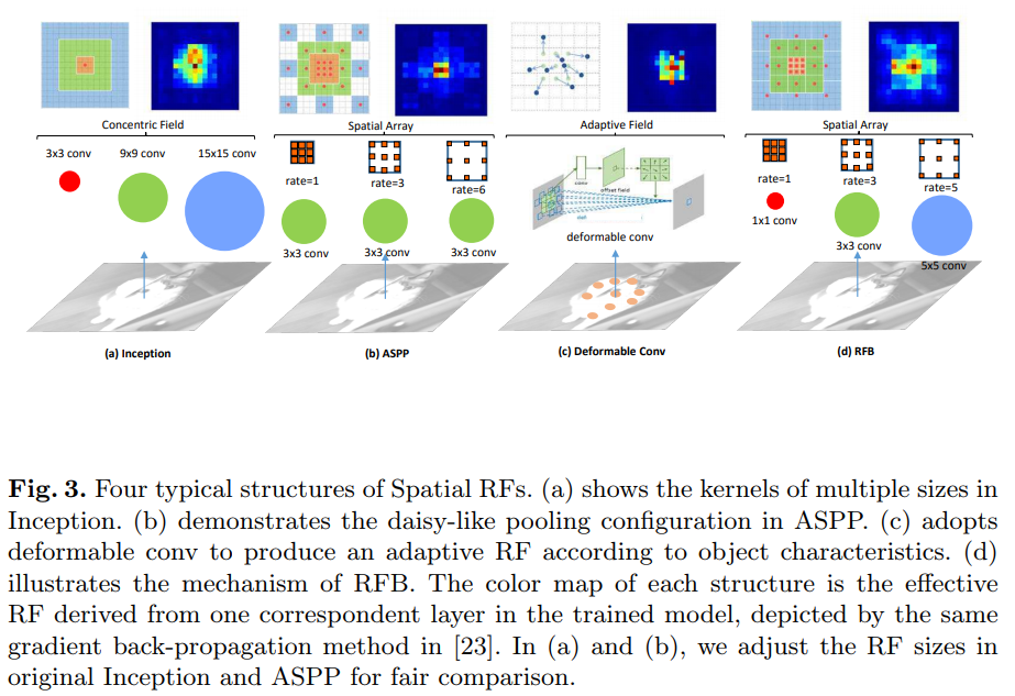
• Inception block은 다른 커널 사이즈를 갖는 multiple branch를 이용하여 multi-scale information을 담고자 했다. 하지만 모든 커널들은 동일한 중심에서 sampled되어 동일한 sampling coverage를 위해서 더 큰 범위가 필요한 경우에 대해서도 동일한 연산을 해 몇몇의 중요한 details 정보들을 담아내지 못했다. ASPP 의 경우 dilated convolution이 중심에서부터 sampling distance가 변하지만 feature가 같은 커널 사이즈를 갖는 이전의 convolution layer에서 uniform resolution을 가지므로 이로인해 모든 위치에서 중요한 clue(특징점들)을 동일하게 처리해 결국 object와 context 사이의 혼란을 야기시키게 된다. Deformable CNN[4] 는 각 객체에 대해 독특한(distinctive) resolution을 학습하지만, 이는 ASPP와 동일한 단점(downside)을 갖게된다. RFB는 앞의 ASPP와 Deformable CNN과는 다르게 daisy-shape configuration에서 RF의 eccentricity(편심)과 size 사이의 관계를 강조하므로(highlight) 작은 kernel일수록 더 큰 weight가 중심에 가까운경우에 대해 더 크게 할당되게 되며, 이로인해 멀리있는것보다 중심에 가까운게 더 중요한 정보임을 알 수 있게 되는것이다. Figure 3에서 다양한 전형적인 spatial RF 구조 차이를 볼 수 있다. 반면에 Inception과 ASPP는 성공적으로 one-stage detector에 적용시키지 못하였으나, RFB에서는 그들의 연구에서 얻어진 장점을 이 문제 해결을 위해 성공적으로 적용시킬 수 있었다.

3 Method

• 본 섹션에선 인간의 visual cortex를 다시 설명하면서 제안하는 RFB component와 이러한 메카니즘이 어떻게 동작하는지 설명하고, RFB Net detector의 구조와 모델 학습/테스트 방법에대해 묘사한다.

3.1 Visual Cortex Revisit

• During the past few decades, it has come true that functional Magnetic Resonance Imaging (fMRI) non-invasively measures human brain activities at a resolution in millimeter, and RF modeling has become an important sensory science tool used to predict responses and clarify brain computations. Since human neuroscience instruments often observe the pooled responses of many neurons, these models are thus commonly called pRF models [36]. Based on fMRI and pRF modeling, it is possible to investigate the relation across many visual field maps in the cortex. 각 cortical map에서 연구자들이 pRF의 사이즈의 편심(eccentricity) 사이의 positive correlation을 발견했으며[36], Figure 1에서처럼 visual field maps에서 이러한 correlation coffeicient가 변화하게 된다.

3.2 Receptive Field Block

• 제안하는 RFB는 multi-branch convolutional block이다. 내부 구조는 두 부분으로 구성되어 있으며, 하나는 다른 커널들을 사용하는 multi-branch convolution layer이고 나머지 하나는 trailing dilated pooling이나 convolution layer들이다. Multi-branch convolution layer 부분은 Inception과 동일하며, 다양한 사이즈의 pRF들을 시뮬레이션하기위한 역할을 한다. 그리고 trailing dilated pooling/conv layer의 경우 인간 시각체계의 pRF 크기와 편심(eccentricity) 사이의 관계를 다시 만들어낸다. Figure 2는 RFB가 해당하는 spatial pooling region maps를 나타낸다.
• Multi-branch convolution layer: CNN의 RF의 정의에 따르면, fixed sized RF를 사용하는것보다 multisize RFs를 사용하는것이 성능이 더 우수하며 multisize RFs를 얻기 위해 서로 다른 크기의 kernel을 적용한다.
• Inception V4와 Inception-ResNet V2[31]과 같은 최신논문의 방법을 적용시켰다. 더 자세히 말하자면, 우선 1x1 conv-layer로 구성된 각 branch에 bottleneck structure를 적용하였으며 이로인해 각 feature map에서 nxn conv-layer 채널수가 줄어들게 된다. 두번째로 5x5 conv-layer를 두 개의 3x3 conv-layer를 쌓아 대채하였으며 이로인해 파라미터 수를 줄이면서도 non-linear layer수를 늘릴 수 있었다. 동일한 이유로 1xn과 nx1 conv-layer를 이용하여 원래의 nxn conv-layer를 대채하였다. 또한 논문에선 ResNet[11]과 Inception-ResNet V2 [31]의 shortcut design을 적용했다.
• Dilated pooling or convolution layer: 이에 대한 개념은 원래 Deeplab[2]에서 astrous conv-layer로 설명되었다. 기본적인 목적은 고해상도의 feature map이 더 많은 context 정보를 넓은 범위에 대해 저장하게 하도록 하면서도 파라미터수를 유지하는 것이다. 이 구조는 semantic segmentation[3]과 같은 task에 대해 검증되었으며, 또한 SSD[22]나 R-FCN[17]과 같은 object detection task에 대해서도 속도나 정확도를 향상시키며 그 효과가 검증되었다.

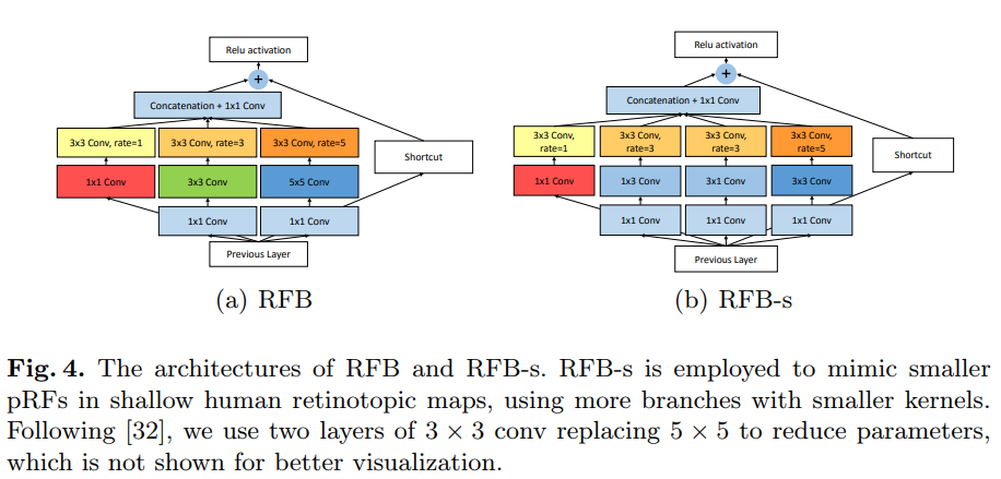
• 본 논문에선 dilated convolution을 human visual cortex의 pRFs의 eccentricity의 impact를 시뮬레이션하기위해 적용하였다. Figure 4는 multi-branch convolution layer와 dilated pooling/convolution layer의 두가지 조합을 보여준다. 각 branch에서 특정한 kernel size를 갖는 conv layer는 해당 dilation이 사용되는 pooling/conv layer를 따른다. 커널 크기와 dilation은 visual cortex의 pRF의 크기와 eccentricity과 비슷한 긍정적인 기능적 관계를 가진다. 결국 모든 branch들의 feature map들은 concat되며, Figure 1에서처럼 spatial pooling이나 convolution array로 합쳐진다.
• 커널 크기, 각 branch의 dilation, 브랜치 수와 같은 특정한 RFB 파라미터들은 detector의 위치에 따라 조금씩 차이가 있으며 이는 다음 섹션에서 다뤄진다.

3.3 RFB Net Detection Architecture

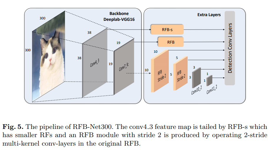
• 제안하는 RFB Net detector는 SSD[22]의 multi-scale, one-stage framework를 이용하며 RFB module이 lightweight backbone이 만들어낸 feature가 detector가 더 정확하지만 여전히 빠르게 동작하도록 한다. RFB가 CNN에 적용이 용이했기 때문에 SSD의 구조를 최대한 원형상태로 유지시켰다. 변경된점은 최상단 conv layer를 RFB로 대채하였으며, 몇몇의 minor하지만 active한 변경들에 대해서 figure 5에서 보여진다.
• Lightweight backbone: SSD와 정확히 동일한 backbone을 썼다. 간단히 ILSVRC CLS-LOC dataset[27]에 pre-trained 된 VGG16[30]의 fc6, fc7 layer를 sub-sampling parameter가 포함된 convolution layer로 바꾸고 pool5 layer를 2x2-s2에서 3x3-s1로 변경시켰다. Dilated convolution layer는 holes를 채우기위해 사용되어지며 dropout layer와 fc8 layer는 제거되었다. 다양한 lightweight network가 존재하지만(DarkNet[25], MobileNet[12], ShuffleNet[39]) 원래의 SSD와 이 backbone에 대한 직접적 비교를 위해 이러한 세팅으로 실험했다.
• RFB on multi-scale feature maps: SSD[22]에서 base network에 conv layer가 cascade되어있어 점점 공간방향 해상도가 감소하고 view field가 증가하는 feature map이 만들어진다. 본 implemenatation에서는 동일한 SSD의 cascade 구조는 유지하지만 앞의 비교적 large resolution의 feature map을 갖는 conv layer들을 RFB module로 바꾼다. RFB 기본버전에선 eccentricity의 효과를 흉내내도록 하는 single structure setting만 사용한다. pRF의 size와 eccentricity 비율은 visual map마다 다르므로 그에맞게 RFB의 파라미터를 조절하여 RFB-s 모듈을 만들었으며 RFB-s는 shallow human retinotopic map의 더 작은 pRFs를 모방하도록 하며 이를 conv4_3 feature 뒤에 넣었다.(Figure 4, 5) 마지막 몇몇 conv layer들은 그대로 형태가 유지되는데 이는 만들어지는 각 feature map이 5x5 커널사이즈 연산을 적용하기엔 너무 작기 때문이다.

3.4 Training Settings

• Pytorch를 이용하였으며, ssd.pytorch repository 코드를 응용했다. 학습전략은 SSD와 대부분 유사하며, data augmentation, hard negative mining, scale and aspect ratios for default boxes, and loss functions (e.g., smooth L1 loss for localization and softmax loss for classification)등은 따르면서 더 나은 RFB 성능을 위해 learning rate schedule은 조정했다. 더 자세한 details는 아래에서 보여진다. 모든 새로붙은 conv layer는 MSRA method[10]로 초기화되었다.

4 Experiment

• We conduct experiments on the Pascal VOC 2007 [5] and MS COCO [21] datasets, which have 20 and 80 object categories respectively. In VOC 2007, a predicted bounding box is positive if its Intersection over Union (IoU) with the ground truth is higher than 0.5, while in COCO, it uses various thresholds for more comprehensive calculation. The metric to evaluate detection performance is the mean Average Precision (mAP).

4.1 Pascal VOC 2007

• In this experiment, we train our RFB Net on the union of 2007 trainval set and 2012 trainval set. We set the batch size at 32 and the initial learning rate at $10^{−3}$ as in the original SSD [22], but it makes the training process not so stable as the loss drastically fluctuates. 대신에 warmup 전략을 사용하여 learning rate를 $10^{-6}$부터 $4\times 10^{-3}$까지 첫 5epoch동안 늘렸다. warmup 이후 원래의 learning rate schedule로 돌아가 150과 200 epoch에서 0.1배 되어진다. 전체 epoch는 250이다. Following [22], we utilize a weight decay of 0.0005 and a momentum of 0.9.

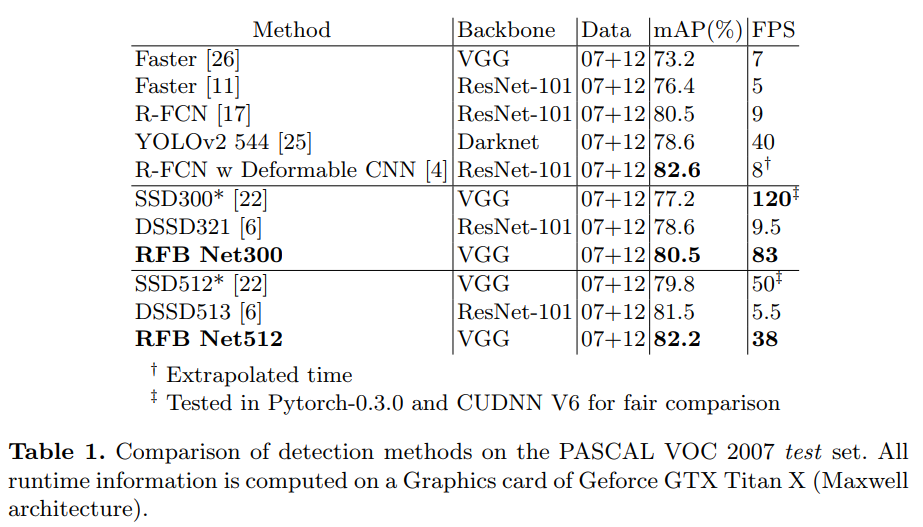
• Table 1은 여러 모델과 VOC 2007에 대한 실험결과 비교를 보여준다. SSD300*과 SSD512*는 [22]에서 학습시 더 많은 작은 객체를 만들기 위해 data augmentation이 적용된 결과이다. For fair comparison, we reimplement SSD with Pytorch-0.3.0 and CUDNN V6, the same environment as that of RFB Net. RFB layer를 합칠 때 basic RFB Net300의 경우 SSD와 YOLO보다 80.5mAP로 더 정확했으며 속도는 SSD300과 같이 real time이 가능한 수준이었다. 심지어 R-FCN[7]과 동일한 정확도이며 two-stage framework를 넘어서는 결과다. RFB Net512의 경우 82.2mAP로 더 큰 input을 받아 매우 깊은 base backbone을 가진 two-stage 모델들보다 정확했으며 동작속도도 빨랐다.

4.2 Ablation Study

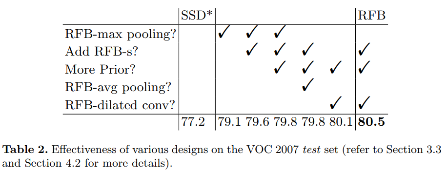
• RFB module: RFB를 더 잘 이해하기 위해 각 component의 영향력에 대해 연구했고 몇몇 비슷한 구조와 RFB를 비교했다. 실험결과는 Table 2와 Table 3에서 보여진다. Table 2에서 볼 수 있듯이 SSD300 with new data augmentation 모델은 77.2mAP를 갖는다. 간단히 conv layer를 RFB-max pooling으로 대채함으로써 성능이 1.9mAP 향상된 79.1mAP까지 좋아진것을 알 수 있으며, 이는 RFB module이 detection에 효과적이라는 것을 의미한다.
• Cortex map simulation: Section 3.3에서 설명되어있듯이 RFB 파라미터들을 cortex maps의 pRF의 size와 eccentricity 사이의 비율을 시뮬레이션하기위해 조절했다. 이러한 tune으로 인해 RFB max pooling의 성능이 0.5mAP, RFB dilated conv가 0.4mAP 개선되었으며 이로인해 human visual system의 메카니즘이 효과있음이 검증된다(table 2).
• More prior anchors: 원래 SSD는 conv4_3, conv10_2, conv11_2 feature map 에서 4개의 default box를, 다른 레이어에선 6개의 default box를 갖는다. [13]에서는 low level feature들이 작은 객체를 찾는데에 매우 중요하다고 한다. 따라서 성능향상을 위해, 특히 작은 객체를 잘 찾기 위해 conv4_3과 같은 low level feature map에 더 많은 anchor를 사용하도록 하였다. 이 실험에서는 conv4_3에 6종류의 default prior를 original SSD에 추가했지만 효과가 없었고, RFB model의 경우 0.2mAP 개선을 얻을 수 있었다.
• Dilated convolutional layer: 초기 실험에서 RFB의 dilated pooling layer를 파라미터 수 증가를 피하기 위해 적용하였지만 이러한 stationary(변하지않는)한 pooling strategy들은 다양한 사이즈의 RFs의 feature fusion을 제한시킨다는 단점이 존재한다. Dilated convolutional layer를 적용시킬 경우 0.7mAP가 향상되었으며, inference time의 증가는 없었다(table 2).
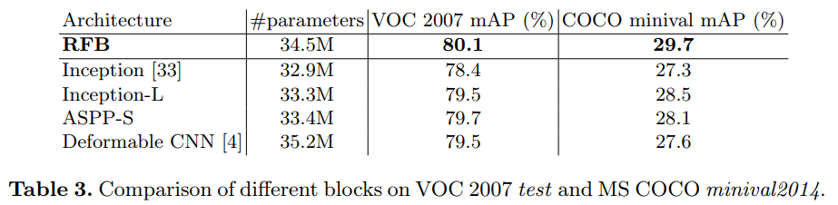
• Comparison with other architectures: 또한 RBF를 Inception, ASPP[3], Deformable CNN[4]과 비교했다. Inception의 경우 RFB와 동일한 RF size를 갖도록 파라미터를 조절하였다. ASPP의 경우 image segmentation[3]을 위한 파라미터들이기에 detection을 하기엔 RFs가 너무 컸다. 따라서 실험에선 RFB와 동일한 RF를 갖도록 조절하였으며 이를 ASPP-S라 칭한다. Figure 3에서 각 방법간의 구조적 차이를 보여준다. 간단하게 이러한 구조들을 detector의 top에 달아놓았으며 Figure 5에서 확인 가능하다. 또한 동일한 학습방법을 적용하고 파라미터수를 최대한 동일하게 하였다. 평가는 Table 3에서처럼 VOC 2007과 COCO에 대하여 수행되었고 RFB의 성능이 가장 좋은것을 확인 할 수 있다. 이는 RFB구조가 detection precision을 높히는데 효과가 있으며, 다른 모델에 비해 더 크고 효율적인 RF를 갖는다.

4.3 Microsoft COCO

• 실험엔 trainval35 셋을(train set + val 35k set) batch size 32로 해서 사용했다. 원래의 SSD 학습전략을 사용하며(COCO에는 VOC보다 객채의 크기가 작으므로 default box의 사이즈를 줄임) 학습시켰다. 학습에는 warmup을 적용하여 5epoch동안 learning rate를 $10^{-6}$부터 $2\times 10^{-3}$까지 증가시켰으며, 다음으로 80epoch와 100epoch에서 10배씩 줄인 후 120epoch에서 학습을 마쳤다.
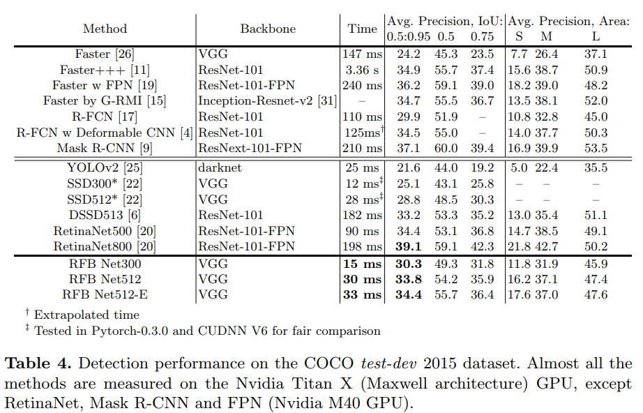
• From Table 4, it can be seen that RFB Net300 achieves 30.3%/49.3% on the test-dev set, which surpasses the baseline score of SSD300* with a large margin, and even equals to that of R-FCN [17] which employs ResNet-101 as the base net with a larger input size (600×1000) under the two stage framework.
• Regarding the bigger model, the result of RFB Net512 is slightly inferior to but still comparable to the one of the recent advanced one-stage model RetinaNet500 (33.8% vs. 34.4%). However, it should be noted that RetinaNet makes use of the deep ResNet-101-FPN backbone and a new loss to make learning focus on hard examples, while our RFB Net is only built on a lightweight VGG model. On the other hand, we can see that RFB Net500 averagely consumes 30 ms per image, while RetinaNet needs 90 ms.
• RetiNet800[20]의 top accuracy 39.7%는 800pixel이라는 매우 높은 resolution을 갖는 input 때문에 얻어졌다. 큰 input이 들어갈수록 보통 성능이 더 좋아지므로 본 논문의 연구에서는 벗어나는 내용이다. 대신 두 가지의 효율적인 update를 고려했다. (1) RFB-s module 적용 전에 conv7_fc의 feautre를 upsample하여 conv4_3의 feature와 concat하여 FPN[19]와 비슷한 효과를 이끌어냈으며, (2) RFB layer에 7*7 kernel을 갖는 branch를 추가하였다. Table 4에서 이로인해 성능이 향상되어 제일 높은 정확도를 보이며, 연산량은 크게 증가하지 않았다. 이 모델의 이름은 RFB Net512-E로 명명된다.

5 Discussion

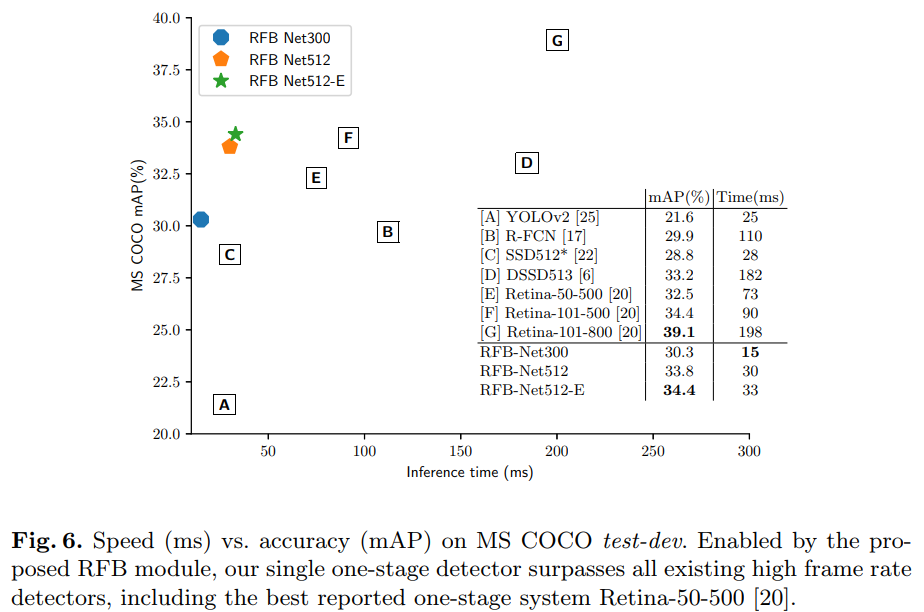
• Inference speed comparison: Table 1과 figure 6에서 다른 top-performing detector들과의 속도를 비교했다. 본 실험에선 다른 dataset에 대한 inference speed가 약간 달랐는데, 이는 MS COCO가 80개의 category가 있고 instance의 평균적인 밀도가 높아 NMS에서 시간이 더 걸리기 때문이다. Table 1에서 RFB Net300이 real-time detector들중 가장 정확하고 PASCAL VOC에 대해 83fps로 동작하였으며, RFB Net512의 경우 더 정확하면서 38fps로 동작했다. Figure 6에서, [20]의 방법대로 speed/accuracy trade-off curve를 MS COCO test-dev set에 대하여 RFB Net과 RetinaNet[20], 다른 모델들에 대해 plot해놓았다. This plot displays that our RFB Net forms an upper envelope among all the real-time detectors. In particular, RFB Net300 keeps a high speed (66 fps) while outperforming all the high frame rate counterparts. Note that they are measured on the same Titan X (Maxwell architecture) GPU, except RetinaNet (Nvidia M40 GPU).

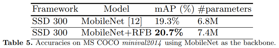
• Other lightweight backbone: 실험에 사용한게 VGG16 이지만 MobileNet[12], DarkNet[25], ShuffleNet[39]등과 비교해 여전이 많은 파라미터를 갖는다. RFB module의 일반화 성능을 테스트하기위해 RFB를 MobileNet-SSD[12]에 적용했다. 해당 모델을 [12]에 따라 MS COCO train+val35k dataset을 동일한 schedule로 학습시켰고 minival로 평가했다. Table 5는 RFB가 MobileNet backbone에도 효과가 있었으며 파라미터의 증가도 매우 적었다. 이는 low-end device의 적용에도 좋은 영향을 끼친다.
• Training from scratch: We also notice another interesting property of the RFB module, i.e. efficiently training the object detector from scratch. [28]과 같은 최근 연구에선 pre-trained backbone을 사용하지 않은 학습방법은 어려운일이며 실제로 처음부터 학습한 모델의 결과가 2-stage로 학습된 결과(pre-trained 사용된 모델)보다 정확도가 더 좋지 못하다. DSOD[28]은 pre-training 모델 없이 VOC 2007에 대해 77.7mAP의 정확도를 갖는 lightweight 구조를 제안했으나 pre-trained 모델을 사용했을 때의 성능 개선이 존재하지 않았다. 논문에선 RFB Net300을 VOC07+12 trainval에 대해 처음부터 학습시켰고 그 결과 77.6mAP를 얻었다. 이는 DSOD 방법과 견줄만한 결과다. 또한 pre-trained 모델을 사용하면 정확도가 80.5mAP까지 개선이 가능하다.

Conclusion

• 본 논문에서는 빠르지만 정확한 object detector를 제안했다. 일반적으로 backbone의 성능 의존도가 높은 모델들에 비해 인간 시각체계의 Receptive Field를 본딴 Receptive Field Block을 적용함으로써 lightweight network의 feature 표현력을 좋게 할 수 있었다. RFB는 RFs의 size와 편심(eccentricity) 사이의 관계를 측정하여 더 discriminative(구별잘하는) 하고 robust한 feature를 생성시킨다. RFB는 lightweight CNN based SSD의 앞부분에 장착되어지며 이로인해 PASCAL VOC와 MS COCO dataset에 대해 엄청난 성능의 향상을 보일 수 있었고, 최종 정확도는 심지어 현존하는 top-performing deeper model based detector를 넘어설 수 있었다. 또한 이를통해 lightweight model의 속도는 유지하면서도 정확도는 향상시킬 수 있었다.