Searching for MobileNetV3

Original paper: https://arxiv.org/pdf/1905.02244.pdf

Authors: Andrew Howard, Mark Sandler, Grace Chu, Liang-Chieh Chen, Bo Chen, Mingxing Tan, Weijun Wang, Yukun Zhu, Ruoming Pang, Vijay Vasudevan, Quoc V. Le, Hartwig Adam (Google)

Abstract

• 새로운 아키텍쳐를 적용시키는 등의 여러 상호 보완적인 기술들을 조합해서 MobileNet v3를 제안
• MobileNet v3는 mobile phone CPU에 최적화되어있음
  • NetAdapt와 NAS를 조합해서 새로운 구조를 제안
• 본 논문에서는 automated search 알고리즘과 네트워크 디자인이 어떻게 같이 동작해서 전체적인 SOTA 성능을 달성하는지에 대한 보완적인 방법들을 다룸
• 그 과정에서 MobileNetV3-Large와 MobileNetV3-Small이라는 모델을 제안함
  • Large는 high resource 사용시, Small은 low resource 사용시
• 위 두 모델들은 Object detection과 Semantic segmentation에 적용되어 테스트 됨
• Semantic segmentation(or any dense pixel prediction)에서는 효율적인 새로운 segmentation decoder인 Lite Reduced Atrous Spatial Pyramid Pooling (LR-ASPP)를 제안함
• Mobile환경에서의 classification, detection, segmentation task에서 SOTA 성능을 달성했음
• MobileNetV3-Large는 MobileNetV2에 비해 ImageNet classification에서 3.2% 정확하면서도 20%의 latency가 개선됨
• MobileNetV3-Small은 MobileNetV2에 비해 비슷한 latency로 6.6% 더 정확했음
• MobileNetV3-Large는 MobileNetV2에 비해 MS COCO detection에서 25% 빠르면서도 비슷한 정확도를 보였음
• MobileNetV3-Large LR-ASPP는 MobileNetV2 R-ASPP에 비해 Cityspace segmentation에서 34% 빠르면서도 비슷한 정확도를 보였음

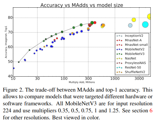
• 위의 figure 2는 MAdds에 따른 top-1 accuracy trade-off를 보여줌
  • 각 모델의 input은 224 resolution을 이용함
  • 각 점들은 0.35, 0.5, 0.75, 1, 1.25의 multiplier를 의미함
• 제안하는 방법이 전반적으로 연산량도 적으면서 정확도가 높은 것을 확인 할 수 있음

1. Introduction

• 효율적인 on-device 인공신경망은 mobile 적용 시대에 있어서 매우 흔함
  • 이러한 on-device 딥러닝은 사용자의 개인정보를 서버로 전송하지 않고도 사용자에 최적화된 구동을 위해 필수로 필요한 분야
  • On-device를 가능하게 하는 효율적인 구조들은 높은 정확도와 적은 latency와 함께 효율적인 구동으로 인해 mobile device의 battery life를 늘려줌
• 본 논문에선 on-device computer vision을 강화하기 위해 더 정확하고 효율적인 MobiletNetV3 Large와 Small 모델들을 제안함
• 논문에서 제안하는 네트워크는 SOTA 성능을 뛰어넘었으며 automated search와 새로운 아키텍처에 결합해 효과적으로 새로운 모델을 구축하는 방법을 설명
• 논문의 목표는 accuracy-latency 최적화를 통해 mobile환경에서 최고의 mobile computer vision architecture를 제안하는 것
• 이를 위해 다음의 것들을 설명
  1. Complementary search techniques
  2. Mobile setting에 효율적인 새로운 non-linearities practical version을 제안
  3. 새로운 효율적인 네트워크 디자인
  4. 새로운 효율적인 segmentation decoder
• 위의 것들을 mobile phone에서 다양하고 광범위한 방법으로 효율성등을 실험적으로 검증함
• 아래의 흐름을 따름
  • Section 2에선 related work에 대해서 다룸
  • Section 3에선 mobile model들의 efficient building block들에서 사용된 방법들을 리뷰
  • Section 4에선 NAS와 MnasNet, NetAdapt 알고리즘들의 상호적인 보완적 특성을 다룸
  • Section 5에선 joint search를 통해 찾아진 모델의 효율을 높히는 새로운 architecture design을 설명
  • Section 6에선 classification, detection, segmentation task를 이용해 모델의 효율과 각 적용요소들의 contribution에 대해 실험하고 결과를 설명
  • Section 7에선 결론 및 future work를 다룸

2. Related Work

• 최근 다방면에서 뉴럴넷의 최적의 정확도-효율 trade-off를 찾기위한 다양한 연구들이 수행됨
  • Hand-crafted 구조들과 NAS를 이용해 찾아진 구조들 모두 이 분야의 연구를 위해 주요하게 사용됨
• SqueezeNet[22]은 squeeze와 expand 모듈과 1x1 컨벌루션을 광범위하게 사용해 파라미터 수를 줄이는것에 중점을 두고 연구되었음
  • 최근에는 파라미터 수를 줄이는 것 뿐만 아니라 실질적인 latency를 줄이기 위해 연산량(MAdds)을 줄이기 위한 연구가 수행됨
• MobileNetV1[19]은 연산 효율 증가를 위해 depthwise separable convolution을 사용함
• MobileNetV2[39]은 위의 방법을 이용하면서도 resource-efficient한 inverted residual block과 linear bottleneck을 제안함
• ShuffleNet[49]은 group convolution과 channel shuffle 연산을 활용해 연산량을 줄임
• CondenseNet[21]은 모델 학습단에서 group convolution을 학습시켜 feature 재사용을 위한 layer간 dense connection을 활용했음

• ShiftNet[46]은 연산비용이 비싼 spatial convolution을 대체하기 위해 point-wise convolution을 중간에 끼워넣은 shift operation을 제안함

• 강화학습을 이용한 NAS로 찾아진 효율적이면서도 competitive한 정확도를 갖는 architecture design들이 있음[53, 54, 3, 27, 35]
• A fully configurable search space can grow exponentially large and intractable.
• 따라서 초기 NAS 연구들은 cell level structure에 집중되었으며, 이로인해 같은 cell들이 모든 layer들에서 재사용되는 구조를 가졌음
• 최근 [43]과 같은 연구에선 block-level의 계층적인 search space에 대해 연구하며 다른 layer structure를 다른 resolution block에서 사용 가능하게 했음
• 네트워크 탐색 과정의 연산비용 감소를 위해서 [28, 5, 45]등에선 gradient based optimization이 적용된 differentiable architecture search framework가 사용되었음

• 또한, 현존하는 네트워크를 강제로 mobile platform에 최적화 시키기 위해 [48, 15, 12]에서는 더 효율적인 automated network simplification algorithm들을 제안함

• [23, 25, 47, 41, 51, 52, 37]에선 양자화(quantization)라는 또다른 complementary effort를 적용시켜 precision arithmetic을 줄여서 네트워크를 효율화시킴
• 마지막으로 [4, 17]에서는 지식증류(knowledge distillation)를 이용해 추가적인 complementary method를 제안했으며, 크고 정확한 teacher network를 통해 작고 부정확한 student network의 효율이 향상됨

3. Efficient Mobile Building Blocks

• Mobile model들은 엄청 효율적인 building block들을 이용해 만들어짐
• MobileNetV1[19]은 depth-wise separable convolution을 이용해 일반적인 conv를 대체하는 방법을 제안함
• Depthwise separable convolution은 효과적으로 일반 conv를 factorize했으며, 이는 feature 생성에서 spatial filtering을 분리시킨 결과

• Depthwise separable conv는 두 개의 분리된 layer로 구성되며, spatial filtering을 위한 light weight depthwise convolution과 feature generation을 위한 heavier 1x1 pointwise conv로 구분됨

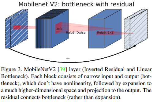
• MobileNetV2[39]은 중요도가 떨어지는 정보의 영향력을 고려해 모델의 효율화를 시킬 수 있는 linear bottleneck과 inverted residual structure를 제안함
• 이 구조는 아래 figure 3에서 확인 가능하며, 이는 depth-wise conv와 1x1 projection layer 뒤에 1x1 expansion convolution으로 구성됨
  • Input과 output은 채널 수가 같은 경우 residual connection으로 연결되게 되어있음
  • 이 구조는 비선형 채널 별 변환의 expressiveness를 높이기 위해 블록 안에서 더 높은 차원의 feature space로 확장시켰고, 이로인해 블록의 입력 및 출력에서 compact한 표현이 유지됨

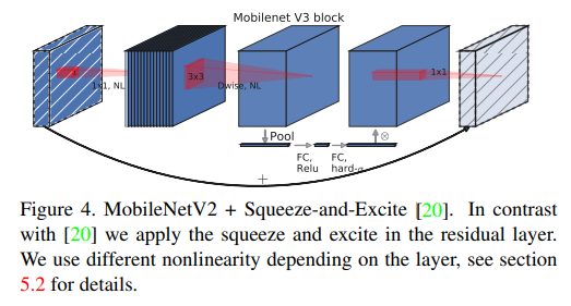
• MnasNet[43]은 MobileNetV2 구조를 기반으로 하는 구조이며, bottleneck 구조에 squeeze and excitation에 기반한 모듈을 제안함.
  • 여기서 squeeze and excitation module은 [20]의 ResNet 기반의 모듈에 다른 위치에서 integrated된 모듈임
• 모듈은 figure 4에서 채널 확장 시의 depthwise filter 뒤에 위치하며, 이는 largest representation에 좀 더 attention을 주기 위함임

• MobileNetV3에선 이러한 방법들의 조합을 building block으로 사용하며, 이는 더 효율적인 모델을 만들기 위함임
• Layer들은 [36, 13, 16]의 swish nonlinearity를 사용하도록 upgrade됨
• 각각 두 squeeze and excitation 또한 swish nonlinearity를 사용했으며, sigmoid는 비효율적인 연산을 대체하면서도 fixed point arthmetic의 정확도 보존을 위해 hard sigmoid[2, 11]을 적용함
  • 자세한 내용은 Section 5.2에서 다뤄짐

4. Network Search

• [53, 43, 5, 48]에선 network search가 새로운 architecture를 찾는 매우 강력한 tool이라는 것을 보여줌
• MobileNetV3에선 각 network block을 최적화하여 global network structure를 찾았으며, platform-aware NAS를 사용함
• 다음으로 NetAdapt 알고리즘을 이용해 layer의 최적의 filter 갯수를 찾음
• 이러한 techniques들은 상호보완적(complementary)이며 주어진 하드웨어 플랫폼 상에서 효율적으로 최적의 조합을 찾기 위해 조합해 사용 가능함

4.1. Platform-Aware NAS for Block-wise Search

• [43]과 유사하게 global network structure를 찾기 위해 platform-aware neural architecture approach를 사용함
• 동일한 RNN-based conwtroller와 같은 factorized hierarchical search space를 사용했기 때문에 [43]과 유사한 결과를 얻었으며, Large mobile model의 target latency는 80ms을 목표로 함

• 따라서 논문에선 MnasNet-A1[43]을 initial Large mobile model로 재사용했으며, NetAdapt[48]과 다른 optimization 방법들을 적용시켜 최적화함

• 하지만 처음에 얻어진 design은 small mobile model에 최적화 되어있지 않았음
• 특히, 이 방법은 multi-objective reward $ACC(m)\times[LAT(m)/TAR]^w$를 Pareto-optimal solution을 근사화하기 위해 사용했음
  • $m$: 생성된 모델
  • $ACC(m)$: 모델의 정확도
  • $LAT(m)$: 모델 latency
  • $TAR$: Target latency
• 하지만, 작은 모델들의 latency와 비교해 정확도가 더 극적으로 변하는것을 확인했음
  • 따라서 latency 변화에 따른 더 큰 정확도 변화를 보완하기 위해 작은 weight factor $w=-0.15$(vs the original $w=-0.07$[43])를 사용함
• 논문의 강화된 새로운 weight factor $w$에 따라 from scratch로 새로운 initial seed model을 NAS를 이용해 찾았으며, 다음으로 NetAdapt와 other opimization 들을 적용시켜 최종적으로 MobileNetV3-Small 을 얻어낼 수 있었음

4.2. NetAdapt for Layer-wise Search

• 저자들이 사용한 다음 기술은 NetAdapt[48].
• 이는 platform-aware NAS에 complimentary(무료)
  • Coarse(조잡한) but global한 architecture를 infer(추론)하지 않고, 순차적으로 개별 레이어를 fine-tuning 할 수 있게 함
  • 자세한 내용은 논문 참조
• 짧게 technique proceed는 아래와 같음
  1. Platform-aware NAS로 찾아진 seed network architecture로 시작
  2. 각 step에서
     • (a) New proposal set을 생성. 각 proposal은 이전 step과 비교해서 latency이 최소 $\delta$ 만큼 감소되는 architecture의 modification을 의미함
     • (b) 각 proposal에 이전 step에서 pre-trained model을 사용하며, 새로 제안 된 architecture를 채우고 누락된 weight를 적절히 자르고 random하게 initialize함. 각 proposal을 $T$ step동안 fine-tuning해서 대략적으로 accuracy를 얻음
     • (c) Some metric을 이용해 최적의 proposal을 선택
  3. 이전 step을 target latency가 얻어질때까지 반복
• [48]에서는 accuracy change를 최소화하는것을 metric으로 사용함
• 본 논문에선 이 알고리즘을 latency change와 accuracy change의 비율을 최소화하도록 바꿈
  • 이는 각 NetAdapt step에서 생성 된 모든 proposal에 대해 $\frac{\delta Acc}{|\delta latency|}$를 최대화 하는 proposal을 선택하도록 함
    • $\delta latency$은 위의 step 2 (a)의 제약사항들을 만족함
    • 저자들들은 직관적으로 제안된 proposal들이 discrete하다고 판단했으므로, trade-off curve의 기울기를 최대화하는 proposal을 선호했음
• 이 과정은 latenct가 target에 도달할때까지 반복되었으며, 다음으로 새로운 모델을 from scratch로 재학습 시킴
• 논문에선 MobileNetV2에서 사용한 [48]의 proposal generator를 사용함
• 특히, 다음의 두 종류의 proposal을 따르도록 함
  1. 모든 expansion layer의 크기를 줄이도록 함
  2. Residual connection을 유지하기 위해 같은 bottleneck size를 갖는 모든 블록들의 모든 bottleneck을 줄임
• 논문의 실험에선 $T=10000$로 했으며, proposal의 초기 fine-tuning의 정확도는 증가되었지만 from scratch로 학습시켰을 때는 최종 정확도는 변하지 않는것을 확인함
• 논문에선 $\delta=0.01|L|$로 설정
  • $L$: seed model의 latency

5. Network Improvements

• 네트워크 탐색에 있어서 최종 모델 향상을 위한 또다른 방법들을 소개함
• 논문에선 네트워크 초기와 끝부분의 연산비용이 비싼 레이어들을 재디자인함
• 또한 새로운 nonlinearity인 h-swish를 제안
  • h-swish는 swish nonlinearity의 modified version으로 연산하기 더 빠르고 양자화-친화적임(quantization-friendly)

5.1. Redesigning Expensive Layers

• NAS로 모델 구조가 찾아진 후 몇개의 초기와 마지막 레이어들이 연산비용이 다른레이어보다 비싼것을 발견함
• 따라서 accuracy는 유지하면서도 latency를 줄이기 위해 몇 modification들을 소개함

• 이 modification들은 현재 search space의 외부적인것

• 첫 번째 modification은 final feature를 더 효율적으로 만들어내도록 네트워크의 마지막 몇 개의 layer가 상호작용(interact) 하도록 재구성 함
• MobielNetV2의 inverted bottleneck 기반의 현재 모델들과 variants들은 1x1 convolution을 final layer로 씀
  • 이는 higher-dimensional feature space로 채널을 확장시키기 위함임
  • 이 layer는 prediction을 위한 충분한(rich) feature를 갖도록 하는 중요한 역할을 함

• 하지만 이는 extra latency라는 문제를 야기함

• 이러한 latency를 줄이고 high-dimensional feature을 보존하기 위해서 해당 레이어를 average pooling 뒤쪽으로 보냄
• 이로인해 그전에는 7x7 spatial resolution으로 연산하는것을 1x1 spatial resoultuion으로 연산하게 되어 연산량이 보존됨

• 이 design choice는 feature 계산이 연산량 및 latency 측면에서 거의 관계가 없기 때문에 적용됨

• Feature generation layer의 비용이 좀 줄어들었기에 이전의 bottleneck projection layer는 computation을 줄일 필요가 없어짐
• 이로인해 이전 bottleneck layer의 projection과 filtering layer를 제거 할 수 있으며, 여기서 또 연산량을 줄일 수 있게 됨
• 원래의 구조와 optimized last stage의 구조는 아래 figure 5에서 확인 가능

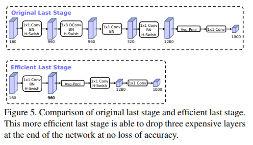
• 효율적인 last stage로 인해 latency를 7ms를 줄일 수 있었으며, 이는 전체 running time의 11%임
  • 정확도의 손실 없이 거의 3천만개(30 millions)의 MAdds를 줄일 수 있었음
  • Section 6에서 자세한 결과를 다룸
• 또다른 expensive layer는 초기 filter set
• 현재 mobile model들은 edge detection을 위한 filter bank를 만들기 위해 3x3 conv와 32개 filter를 사용하는 경향이 있음
  • 종종 이러한 필터들은 서로 mirror 이미지일 수 있음
• 따라서 저자들은 이러한 필터의 redundancy를 줄이기 위해 수를 줄이고 다른 non-linearity들을 적용시켜 봄
• 이미 테스트 된 다른 non-linearity 뿐만 아니라 hard swish nonlinearity를 이 레이어들에 적용시킴
• 이로인해 원래 ReLU나 swish와 32개 filter를 썼을 때와 동일한 정확도로 16개의 filter로 구현 할 수 있었음
  • 이 과정에서 latency 약 2 ms와 천만개(10 million)의 MAdds를 줄일 수 있었음

5.2. Nonlinearities

• [36, 13, 16]에서는 swish라는 nonlinearity가 제안되었으며, 이는 ReLU의 drop-in replacement임
  • 이는 neural network의 정확도를 크게 개선 시켜 줄 수 있음
• Swish는 아래와 같이 정의됨
  • swish $x = x\cdot \rho (x)$
• Swish nonlinearity가 정확도를 향상시키는 반면 sigmoid처럼 모바일 환경에서 계산 할 때의 비용이 큼
  • ReLU의 계산비용은 0
• 따라서 저자들은 이 문제를 두 가지 방법으로 타협함

Method 1

• Sigmoid function을 piece-wise linear hard analog로 바꿈
  • [11, 44]와 유사한 $\frac{ReLU6(x+3)}{6}$로 대체
• [11, 44]와 다른점이라면 custom clipping constant 대신 ReLU6를 사용함
• 유사하게 hard version of swish는 아래와 같음
  • $h-swish[x] = x\frac{ReLU6(x+3)}{6}$
• [2]에선 hard-swish와 유사한 버전이 최근에 제안됨
• Figure 6에선 sigmoid와 swish의 soft와 hard version의 차이를 보여줌

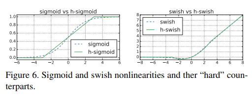
• 사용된 상수는 원래의 smooth version과 잘 맞도록 선택됨
• 논문의 실험에서, 함수들의 hard-version을 사용했을 때 정확도의 차이는 없었지만 deployment 관점에서 몇 장점들이 있었음
  • 우선, 모든 software와 hardware framework에서 사실상 ReLU6의 iptimized implementation이 가능했음
  • 다음으로, 양자화 모드에서, hard-version은 approximate sigmoid의 또다른 implementation으로 인한 potential numerical precisioin loss를 제거함
  • 마지막으로, 실제 h-swish는 piece-wise(간단한) function으로 implementation 될 수 있으므로 latency cost를 크게 낮출 수 있는 memory access 횟수를 줄임

Method 2

• Nonlinearity를 적용하는데 필요한 cost는 네트워크의 깊은 단으로 갈 수록 줄어들게 됨
  • 이는 각 layer activation memory가 일반적으로 resolution이 떨어질 때 마다 반으로 줄어들기 때문
• 동일하게 deeper layer에서 swish를 사용할때만 benefit이 있는걸 확인함
• 따라서 논문의 architecture에선 후반부에만 h-swish를 사용함
• Table 1과 table 2에서 정확한 layout을 확인 가능

• 이러한 optimization에도 h-swish는 아직도 약간의 latency cost를 발생시킴
• 하지만 section 6에서 설명하듯 accuracy와 latency에 대한 순 효과는 최적화 없이도 좋았지만, piece-wise function 기반의 optimized implementation을 사용 할 때 좀 더 좋은 결과를 보였음

5.3. Large squeeze-and-excite

• [43]에서 squeeze-and-excite bottleneck의 크기는 convolutional bottleneck의 크기에 상대적이라고 했음
• 대신에, 본 논문에선 이것들을 expansion layer의 channel의 1/4개로 fix시킴
  • 이렇게 하는게 정확도도 높아지면서 파라미터 수의 증가는 제한 할 수 있었고, 거의 구별 불가능할정도로 조금의 latency cost만 발생함

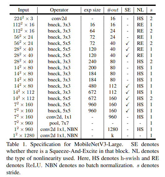
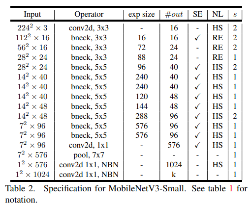
5.4. MobileNetV3 Definitions

• MobileNetV3은 두 개의 모델로 정의됨
  • MobileNetV3-Large
  • MobileNetV3-Small
• 이 모델들은 각각 resource를 많게/적게 사용할 때를 target함
• 모델들은 platform-aware NAS와 NetAdapt를 적용해 만들어졌으며, 이 섹션(section 5)에서 정의 된 네트워크 improvements들을 통합해 만들어짐
• 자세한 내용/구조는 위의 table 1과 2를 참고

6. Experiment

• MobileNetV3의 성능 검증을 위한 다양한 실험을 수행
  • 실험은 classification, detection, segmentation으로 수행
• 또한 다양한 ablation study들을 통해 다양한 design decision들의 영향을 밝힘

6.1. Classification

• ImageNet[38] 데이터셋을 이용해 실험함
  • Accuracy, latency, multiply adds (MAdds) 측정

6.1.1 Training setup

• 논문의 모델을 4x4 TPU Pod[24]에서 synchronous training setup을 이용해 학습시켰으며, standard tensorflow RMSPropOPtimizer with 0.9 momentum을 사용함
• 초기 learning rate는 0.1, batch size는 4096 (128 images per chip), learning rate decay rate는 3epoch마다 0.01로 적용
• 0.8의 dropout, 1e-5의 l2 weight decay과 Inception[42]과 동일한 image preprocessing을 적용
• 마지막으로 decay 0.9999의 exponentail moving average를 사용함
• 모든 convolutional layer들은 batch-normalization layer들을 사용하며 average decay는 0.99로 적용

6.1.2 Measurement setup

• Latency를 측정하기 위해 standard Google Pixel phone을 사용했으며, 모든 네트워크는 standard TFLite Benchmark Tool을 이용해 동작함
• 모든 측정 실험엔 single-threaded large core를 사용함
• 실험에선 multi-core inference time을 측정하지 않았음
  • 이는 mobile application에서 일반적이지 않기 때문임
• 논문에선 atomic h-swish operator를 tensorflow lite에 기여(contribute)했으며, 현재 최신의 tensorflow lite에 default로 적용되어있음
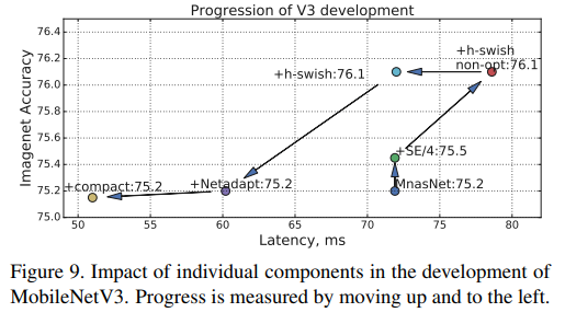
• Figure 9에선 optimized h-swish의 impact를 보여줌

6.2. Results

• 위의 figure 1에서 보여지듯 제안하는 모델이 MnasNet[43], ProxylessNas[5], MobileNetV2[39]과 같은 SOTA 모델들의 성능을 뛰어넘음
• Table 3에선 서로다른 Pixel 폰에서 floating point 연산의 성능을 보여줌

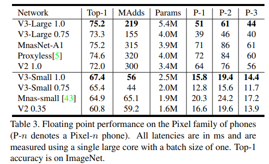
• 위의 table 3은 구글 pixel phone의 1, 2, 3세대에 따른 성능을 보여줌
• 모든 latency는 ms단위이며, single large core with batch size 1의 성능을 보임
• Top-1 ImageNet accuracy를 볼 수 있음
• 제안하는 모델이 가장 빠르면서도 정확하게 동작하는것을 확인 할 수 있음
  • 표에서 모델 옆의 숫자는 MobileNets와 동일하게 width multiplier hyperparameter를 의미하는듯.
• Table 4에선 quantization을 포함시킨 결과를 보여줌

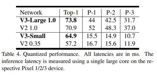
• 위의 table 4에서 모든 latency 단위는 ms를 의미함.
• 위 table 3과 동일하게 각각 구글 픽셀 1, 2, 3에서 single large core 결과를 보여줌.

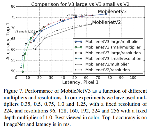
• 위의 figure 7에서, MobileNetV3의 multiplier와 resolution에 따른 성능 trade-off를 볼 수 있음
• 여기서 눈여겨 볼 점은 MobileNetV3-Small이 성능을 맞추기 위해 multiplier가 적용된 MobileNetV3-Large의 성능을 3%가량 앞섰다는 점임
• 반면 resolution은 multiplier보다 더 나은 trade-off를 보여줌
• 하지만, resolution은 대게 task에 의해 결정되므로(예를 들어 segmentation과 detection 문제에선 일반적으로 higher resolution을 필요함) 항상 튜닝 가능한(tunable) 파라미터로 볼 수 없음

6.2.1 Ablation study

Impact of non-linearities

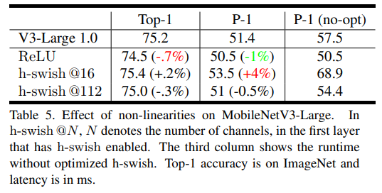
• Table 5에서는 h-swish의 삽입 위치와 naive(vanilla) implementation에 대한 optimized implementation 결과를 보여줌
  • Table 5는 MobileNetV3-Large의 nonlinearity에 대한 영향을 보여줌
  • h-wish@N에서 N은 h-swish가 적용된 첫 번째 레이어의 채널의 수를 의미함
  • 세 번째 column은 optimized h-swish가 없을 때의 runtime을 보여줌
  • ImageNet Top-1 accuracy와 이 때의 latency를 ms단위로 나타냄
• 실험 결과를 볼 때, 최적화 적용된 h-swish가 6ms정도(연산시간의 10%이상)를 줄여주는것을 확인 할 수 있음

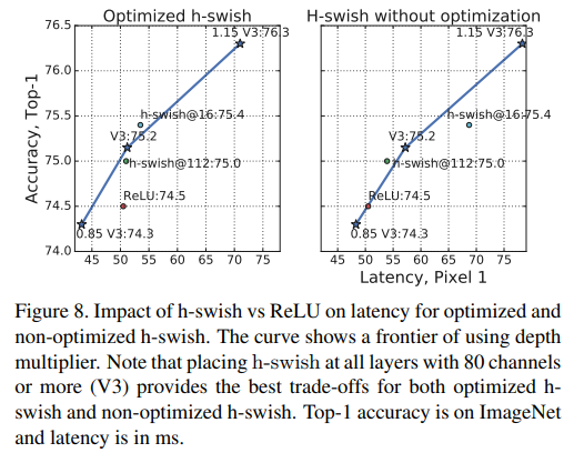
• Figure 8에선 nonlinearity choice와 network width에 의한 효율적인 frontier를 보여줌
  • Figure 8은 최적화 및 최적화 되지 않은 h-swish와 h-swish vs ReLU의 latency를 보여줌
  • Curve는 depth multiplier에 따른 frontier를 보여줌
  • 80개 이상의 채널을 갖는 V3의 모든 레이어에 최적화된 h-swish나 그냥 h-swish를 적용하면 모두 best trade-off를 provide함
  • 표는 Top-1 ImageNet accuracy와 latency를 ms단위로 보여줌
• MobileNetV3은 네트워크 중간부터 h-swish를 사용하며, ReLU의 성능을 확실하게 뛰어넘음
• 단순히 전체 네트워크에 h-swish를 추가하는것만으로도 네트워크를 넓게 하는것보다 성능이 약간 더 좋다는것이 흥미로운 점임

Impact of other components

• Figure 9에선 다른 component들의 적용이 latency와 accuracy의 곡선을 따라 어떻게 변화했는지를 보여줌
  • Figure 9의 그래프는 처음에서 위-왼쪽으로 움직임

6.3. Detection

• 논문의 MobileNetV3을 SSDLitye[39]의 backbone으로 사용했으며, 다른 네트워크들과 MS COCO에서 성능을 비교함
• MobileNetV2에 따라서 SSDLite의 feature extractor의 뒷부분에 첫 번째 layer(output stride 16)와 두 번째 layer(output stride 32)을 추가하고 이를 각각 C4와 C5로 정의함
• MobileNetV3-Large에 대해 C4는 14번째 bottleneck block의 expansion layer로 작용함
• MobileNetV3-Small에 대해 C4는 9번째 bottleneck block의 expansion layer로 작용함
• 두 네트워크에 C5 layer는 pooling 바로 앞에 붙음
• 또한 C4와 C5 사이의 모든 feature layer의 채널 수를 2씩 줄임
• 이는 MobileNetV3의 뒷쪽의 몇 레이어들이 1000개 class를 추론하도록 tune되어있기 때문이며, 이는 COCO의 90개 class 추론을 위한 task에 redundancy로 작용하기 때문임

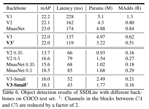
• Table 6는 MS COCO 실험결과를 보여줌
• Channel reduction이 적용되었을 때 MobileNetV3-Large는 MobileNetV2보다 27% 빠르면서도 동일한 mAP 점수를 가졌음
• MobileNetV3-Small with channel reduction 모델은 MobileNetV2와 MnasNet보다 각각 2.4와 0.5mAP가 높으면서도 35% 빠르게 동작했음
• 두 MobileNetV3 모델 모두 channel reduction trick을 적용시켜 15%의 redundancy를 줄이면서도 mAP의 loss는 없었음
  • ImageNet classification과 COCO object detection 모두 다른 feature extractor 모양을 가지면서도

6.4. Semantic Segmentation

• In this subsection, we employ MobileNetV2 [39] and the proposed MobileNetV3 as network backbones for the task of mobile semantic segmentation.
• Additionally, we compare two segmentation heads. The first one, referred to as R-ASPP, was proposed in [39]. R-ASPP is a reduced design of the Atrous Spatial Pyramid Pooling module [7, 8, 9], which adopts only two branches consisting of a 1 × 1 convolution and a global-average pooling operation [29, 50].
• In this work, we propose another light-weight segmentation head, referred to as Lite R-ASPP (or LR-ASPP), as shown in Fig. 10.

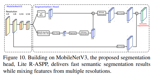
• Lite R-ASPP, improving over R-ASPP, deploys the global-average pooling in a fashion similar to the Squeeze-and-Excitation module [20], in which we employ a large pooling kernel with a large stride (to save some computation) and only one 1×1 convolution in the module.

• We apply atrous convolution [18, 40, 33, 6] to the last block of MobileNetV3 to extract denser features, and further add a skip connection [30] from low-level features to capture more detailed information.

• We conduct the experiments on the Cityscapes dataset[10] with metric mIOU [14], and only exploit the ‘fine’ annotations. We employ the same training protocol as [8, 39].
• All our models are trained from scratch without pretraining on ImageNet [38], and are evaluated with a single-scale input.
• Similar to object detection, we observe that we could reduce the channels in the last block of network backbone by a factor of 2 without degrading the performance significantly.
• We think it is because the backbone is designed for 1000 classes ImageNet image classification [38] while there are only 19 classes on Cityscapes, implying there is some channel redundancy in the backbone.

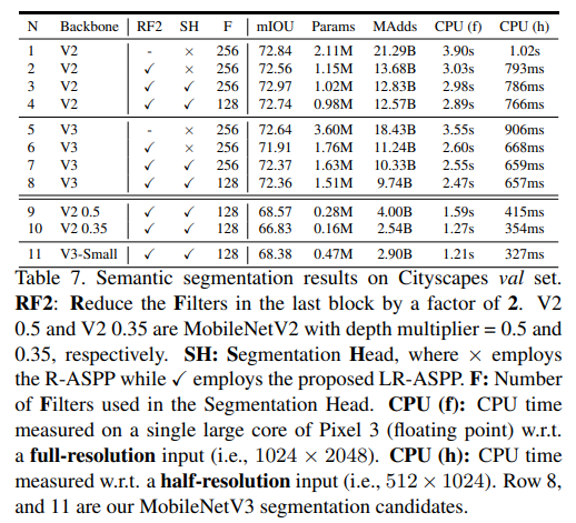
• We report our Cityscapes validation set results in Tab. 7.
• As shown in the table, we observe that (1) reducing the channels in the last block of network backbone by a factor of 2 significantly improves the speed while maintaining similar performances (row 1 vs. row 2, and row 5 vs. row 6), (2) the proposed segmentation head LR-ASPP is slightly faster than R-ASPP [39] while performance is improved (row 2 vs. row 3, and row 6 vs. row 7), (3) reducing the filters in the segmentation head from 256 to 128 improves the speed at the cost of slightly worse performance (row 3 vs. row 4, and row 7 vs. row 8), (4) when employing the same setting, MobileNetV3 model variants attain similar performance while being slightly faster than MobileNetV2 counterparts (row 1 vs. row 5, row 2 vs. row 6, row 3 vs. row 7, and row 4 vs. row 8), (5) MobileNetV3-Small attains similar performance as MobileNetV2-0.5 while being faster, and (6) MobileNetV3-Small is significantly better than MobileNetV2-0.35 while yielding similar speed.

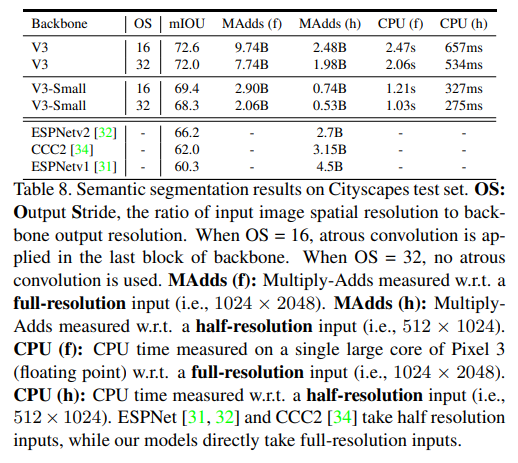
• Tab. 8 shows our Cityscapes test set results.
• Our segmentation models with MobileNetV3 as network backbone outperforms ESPNetv2 [32], CCC2 [34], and ESPNetv1 [32] by 6.4%, 10.6%, 12.3%, respectively while being faster in terms of MAdds. The performance drops slightly by 0.6% when not employing the atrous convolution to extract dense feature maps in the last block of MobileNetV3, but the speed is improved to 1.98B (for half-resolution inputs), which is 1.36, 1.59, and 2.27 times faster than ESPNetv2, CCC2, and ESPNetv1, respectively. Furthermore, our models with MobileNetV3-Small as network backbone still outperforms all of them by at least a healthy margin of 2.1%.

A. Performance table for different resolutions and multipliers

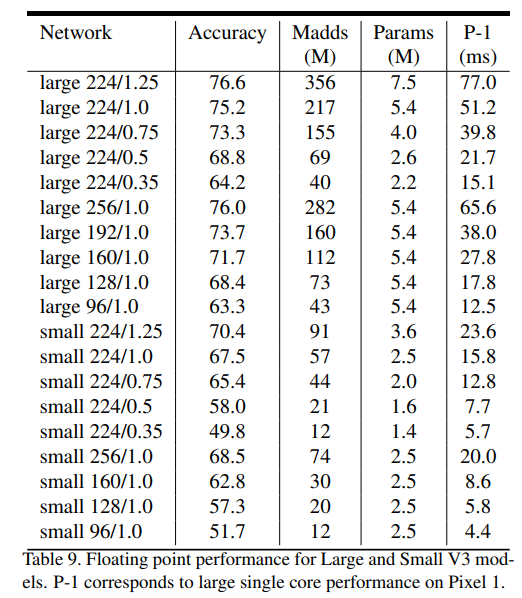
• We give detailed table containing multiply-adds, accuracy, parameter count and latency in Table 9.

7. Conclusion and Future Work

• 본 논문에선 MobileNetV3 Large와 Small 모델을 제안했으며, mobile classification, detection, segmentation에서 SOTA였음
• 논문에선 차세대 모바일용 모델을 제안하기 위해 네트워크 설계 뿐만 아니라 여러 NAS 알고리즘들을 활용함
• Swish와 같은 nonlinearity를 어떻게 최적화하는지 보였으며, quantization friendly(효과적인)한 squeeze and excite를 적용하고 효율성 측면에서 mobile model domain에 적용시킴
• 또한 lightweight segmentation decoder인 LR-ASPP를 제안함
• NAS을 인간의 직관과 가장 잘 혼합하는 방법에 대한 open question이 남아있지만, 저자들은 이러한 question에 대한 첫 번째 긍정적인 결과를 제시함

Summary

• NAS를 이용하여 MNasNet와 MobileNetV2 layer 기반의 MobileNetV3를 제안했음
• Swish nonlinearity를 fixed point 연산에 최적화시킨 hard-swish (h-swish) activation function을 제안
• 기존 방법들 대비 우수한 성능을 보였으며, classification, object detection, semantic sgementation에 적용 시 좋은 성능을 보였음

• Efficient segmtentation을 위한 decoder 구조인 Lite Reduced Atrous Spatial Pyramid Pooling (LR-ASPP)를 제안

• 구글이기에, 이렇게 NAS 실험을 해서 얻을 수 있는.. 효율적인 backbone 구조를 제안하는 논문…